This article describes adjustments that should be made to terminal cash flow that is used to derive terminal value. The adjustments are made to reflect various factors that become stable as the growth rate changes and becomes stable. The general idea is that if there is less growth there should be less investment to support the growth. Various different theoretical ideas and practical formulas can be used to use this idea to compute normalised cash flow in the terminal period that is internally consistent. Adjustments to stable cash flow include stable capital expenditures, stable ROIC relative to WACC, stable deferred taxes and stable working capital all of which depend on the assumed terminal growth rate. For example, if the terminal growth rate in EBITDA is higher, then the amount of investment in inventories is also higher.
Excel File with Demonstration of Formula for Stable Working Capital that Depends on Terminal Growth
This files that you can download above demonstrate issues associated with computing stable working capital changes when you are computing terminal normalised cash flow. The first file is a simple case with only accounts receivable. The second file includes other working capital items and has a bit more detail In evaluating stable working capital both files demonstrate that you can use the following formula in the terminal period for stable working capital:
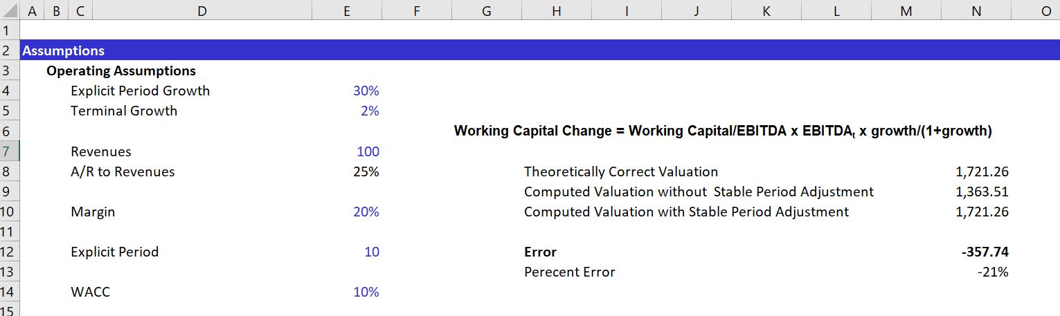
Stable WC Change = WC/EBITDA * EBITDA t * terminal growth/(1+terminal growth).
The screenshot below introduces you to the file and the assumptions. On the right side of the screenshot you can see the magnitude of the error. This depends on the difference between explicit period growth which is very high in the example and the terminal growth. It also depends on the level of working capital relative to the EBITDA. If the margin is low and the working capital is high, the error from not making a terminal value adjustment can be great.
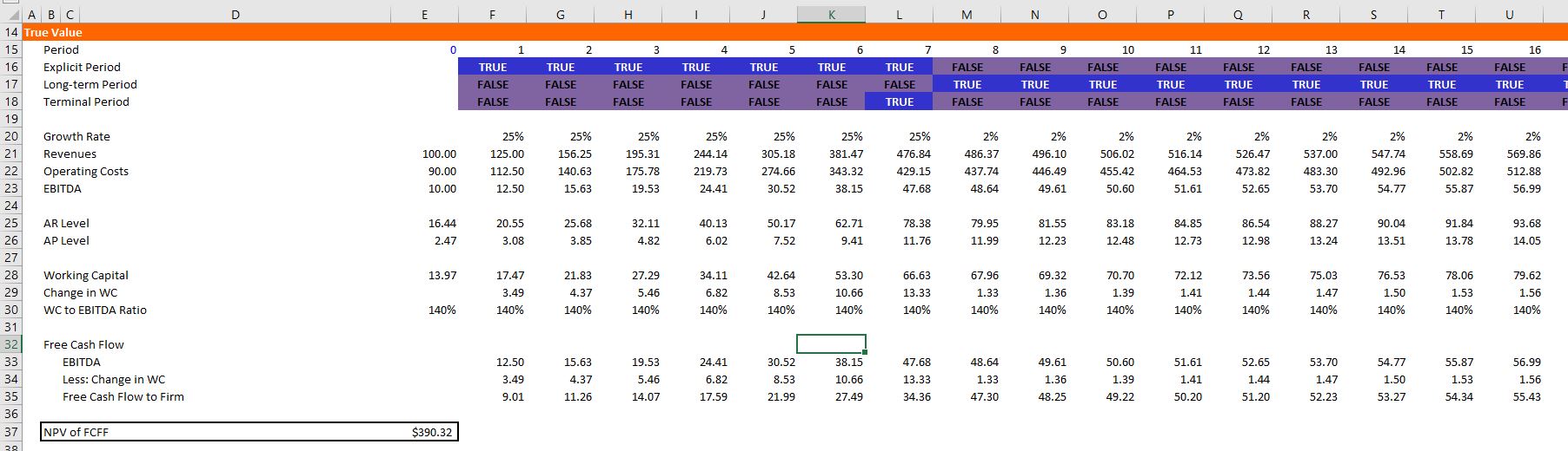
The next screenshot demonstrates the proof of the formula. The model is a forever model that can be used in a proof. When you go out a very long time with growth rate changes you can then see what happens to the true value. After establishing the true value with the very long-term growth, you can develop a model that tests your method. In this case you can put in a terminal value switch and then compute the terminal value using the regular growth method. This is the formula shown in the bar. When you compute the NPV of the cash flows, they do not equal the theoretically correct number.

The next screenshot illustrates the corrected method with a stable working capital ratio. In this case the change in working capital is computed using the formula above and it is dramatically less. When you use the lower number for changes in working capital and then compute the net present value, the result is consistent with the true theoretical number.

File with a little more detail
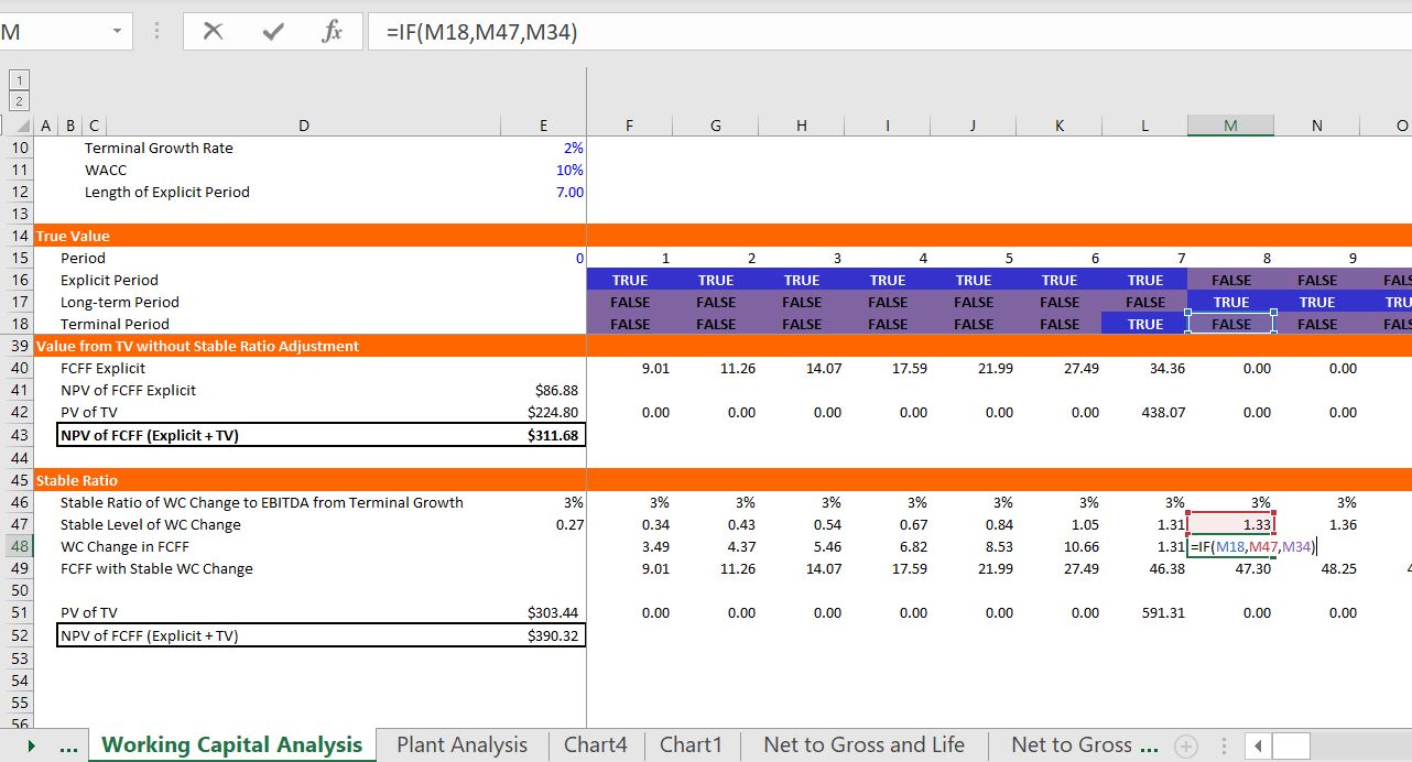
The screenshots below illustrate the same type of analysis for working capital. For this, all that I am really saying is that you do not have to add a second post-terminal period cash flow which can be a pain to compute when you put everything at the terminal growth. Further, this method of including a post-terminal cash flow can lead to problems when you start considering things like capital expenditures and deferred taxes. This file also uses the formula:
Stable WC Change = WC/EBITDA * EBITDA t * terminal growth/(1+terminal growth).

As with the prior file, the analysis and proof begins with a long-term model. You can find more discussion of how to develop proofs in an associated web page. In any of the proofs that I develop, I create a very long term model (consider the contrast between corporate finance and project finance). The valuation over a very long-term period is shown at the bottom of this section.
As with the first example, the final part of the analysis illustrates valuation using a terminal period. The philosophy of the terminal value is that there will be some point when growth becomes stable. If no normalisation adjustment is made, there is undervaluation of the company. The valuation without adjustment is 311. With the corrected working capital adjustment the value becomes 390.
Video Discussion
[wonderplugin_video iframe=”https://www.youtube.com/watch?v=D1WWxM7ZbY0″ videowidth=600 videoheight=400 keepaspectratio=1 videocss=”position:relative;display:block;background-color:#000;overflow:hidden;max-width:100%;margin:0 auto;” playbutton=”http://edbodmer.com/wp-content/plugins/wonderplugin-video-embed/engine/playvideo-64-64-0.png”]
Stable Return on Invested Capital
Cyclical industries
ROI and lumpy investments
Think about the IRR analysis and the difference between ROIC and IRR. When the IRR is different due to age can understand that in the long-run, the IRR and ROIC should be similar.
I am in the process of documenting the various files and uploading the files that were included on my previous website that was suddenly taken down. If you would like the files listed below, please send an e-mail to edwardbodmer@gmail.com and request the resource library.
Stable Ratio Analysis.xlsm
Exercise 4 – Free Cash Flow Exercise.xls
Stable Cap Exp to Depreciation with Historic Growth.xlsm
Stable Working Capital.xlsm
Long-term Proof of Accounts Payable and Cash.xlsm
AP Proof.xlsm
Proofs of Equity Value and Enterprise Value Bridge.xlsm