This page describes how to set-up assumptions efficient way to structure a financial model, including how you may present the assumptions; where to put the assumptions; and how implement alternative mathematical methods of deriving the assumptions. In addition, this page describes some economic theory with respect to creating assumptions and problems with typical discussion of risk. The discussion covers using different time series equations and evaluating the relationship between revenues and different types of costs. The discussion on this page is part of a series of different sections that work through the construction of a corporate model on a step-by-step basis. A crucial part of developing the assumption structure is the magic historic switch. Creating the assumptions section of the model is discussed using selected exercises and documented with associated videos. The file attached to the button below includes historic data for a company. If you work with the exercise file, you should fill in the equations with the yellow background colour.
[wonderplugin_video iframe=”https://youtu.be/Y_qByzoCQ2k” videowidth=600 videoheight=400 keepaspectratio=1 videocss=”position:relative;display:block;background-color:#000;overflow:hidden;max-width:100%;margin:0 auto;” playbutton=”https://edbodmer.com/wp-content/plugins/wonderplugin-video-embed/engine/playvideo-64-64-0.png”]
Assumptions and Economic Theory
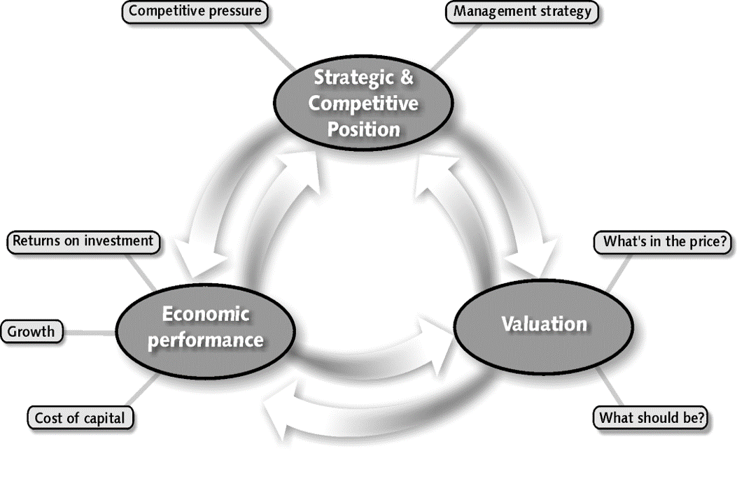
When rating agencies or business school professors discuss assumptions and risks of cash flow, the presentations seem sophisticated and mysterious as illustrated in the screenshot below from Standard and Poor’s (you can find many examples like this from available materials). These are vague and I cannot see how they help anything at all. When you develop assumptions you would like to find potential changes in variables such as the price of the product or the volumes sold or the cost structure and see how much they can vary. The B.S. things from rating agencies like the diagram below say nothing about how variables move. But they are rarely followed by specific examples of how various macroeconomic and industry factors translate into the details of a financial model. After many years of being intimidated I have concluded they are for the most part B.S. The screenshot below illustrates a typical B.S. discussion of risk (and thereby assumptions for a financial model) from S&P. For me, most of these things do not help at all, they are obvious, vague and don not reflect what really happens when businesses turn bad. Instead, you should think about fundamental micro-economic analysis with respect to short-run and long-run marginal costs, demand growth and volatility in an industry, surplus capacity and the really difficult thing, which is predicting changes in tastes, fashions, technology and competitive behavior.
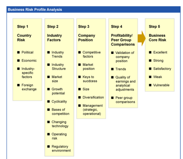
In the above table, the words surplus capacity, differences between short-run and long-run marginal cost, obsolescence, fashion changes, changes in cost structure do not even appear. So I have tried to apply some basic economic principles to risk assessment and assumption development. As I am a negative pessimistic person, when I teach to bankers I really like to hear about bad stories of failures. Here are some of the risks and downsides on my list:
- Surplus capacity from demand in an industry reduction combined with capital intensity and large difference between short-run marginal cost and long-run marginal cost.
- Examples: telecom fiber optic cable, U.S. housing in 2008, shale gas, bulk ships, electricity
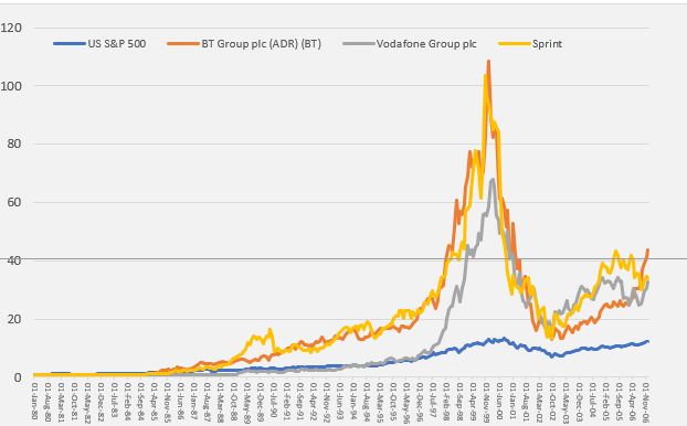
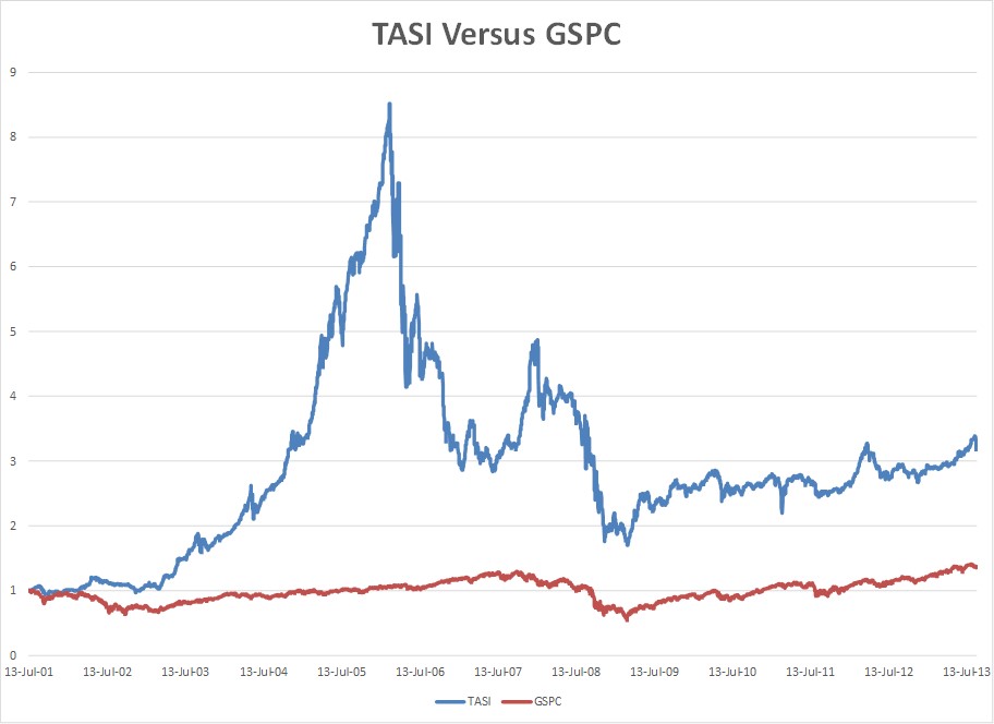
- One of the famous examples of surplus capacity is illustrated by stock prices of telecom companies in the dot.com bubble as shown in the graph below. As the internet was taking off in the 1990’s there companies that had any association with the backbone for the internet were valued very highly. This led to large capital expenditures because companies that had more capital associated with internet operations saw their stock price increase. With the higher capital expenditures, the industry experienced very large surpluses of things like fiber optic cable. Indeed, there was such a massive investment in fiber optic cable that lead to hundreds of years of surplus capacity. Price crashed, and stock prices fell as illustrated in the diagram below.
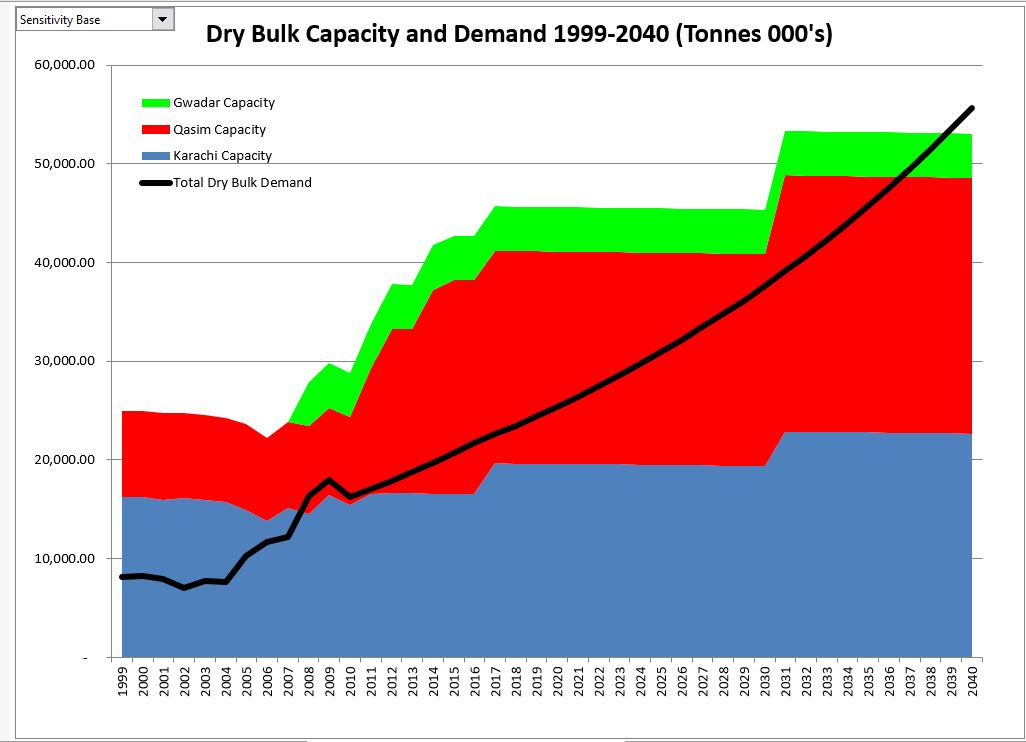
The diagram below is of industry supply and demand for a port in Pakistan. If you can get data on the industry and then you see the dramatic increase in supply relative to demand, this should be a concern. If the demand grows more slowly, the surplus situation will exist for a very long time.
- All sorts of obsolescence, fashion changes, innovation that cause margins to suddenly change and that are very difficult to forecast.
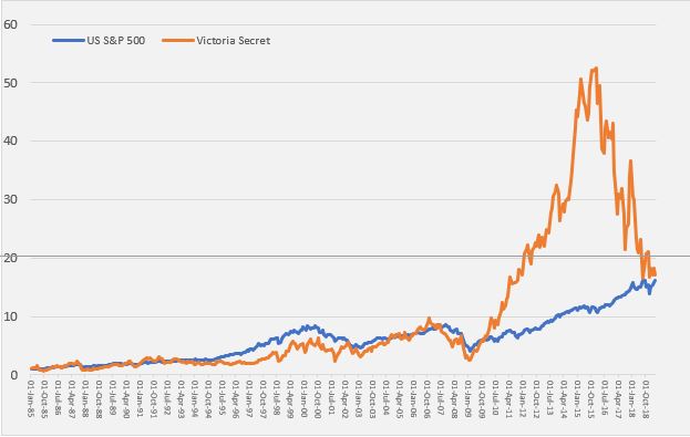
- Examples: Blackberry, Nokia, Victoria Secret, Sears, Kodak, Blockbuster. A graph for Victoria Secret that illustrates difficulties of maintaining fashion is shown below.
- I don’t know how you can forecast things like the problems with Victoria Secret or Blackberry or even retail stores that are subject to competition from Amazon. A couple things to consider are the ROIC compared to ease of entry of other firms and the risk of companies in oligopolistic industries.
- Changing cost structure
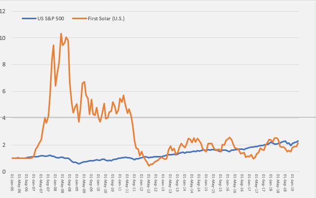
- Examples: solar power, airlines; clothes; furniture. An example of a firm that seemed to be powerful company with high returns and high growth is shown below. For this company in the solar power manufacturing business, there was a dramatic decline in value after the Chinese entered the market in force.
Other factors that are pretty obvious and can cause problems with future cash flow include the following:
- Reliance on uneconomic contracts that cannot be sustained
- Pure fraud in which a lot of money is made and it is very tempting to take the money out
- Inventory obsolescence where the largest investment in assets is stocks and the value can rapidly change
- Reliance on idiotic consultant forecasts and the firehouse effect where people convince themselves that
- Believing in operating leverage where you can grow and increase value through taking advantage of fixed costs
- Is the industry in the middle of a price bubble
Setting-up Assumptions in Model
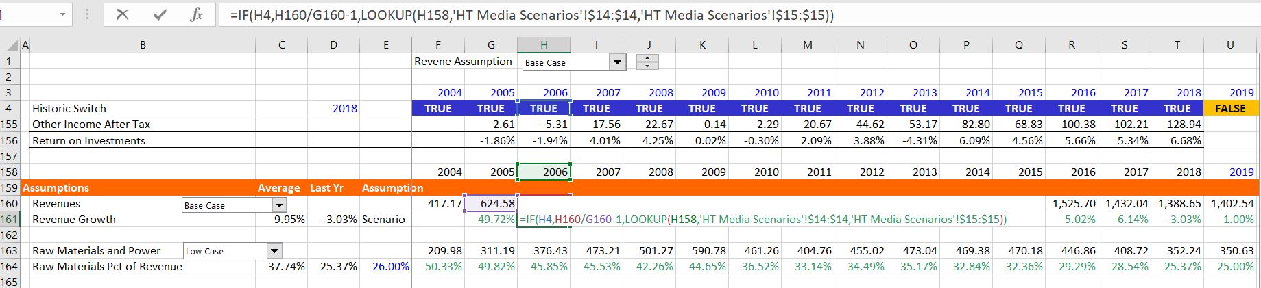
In developing assumptions I think it is essential to begin with a historic switch. This is illustrated in the screenshot below. With this switch you can easily update the model when new financial reports arrive. In the example shown in the screenshot below, the historic switch is in row 4 and the final historic date is 2018. You can change the historic date and the historic switch will change — the formula is simply = year <= last historic year. The screenshot also illustrates the ordering of assumptions beginning with revenues and moving to cost of goods sold. This should conform to the way your model will be constructed.
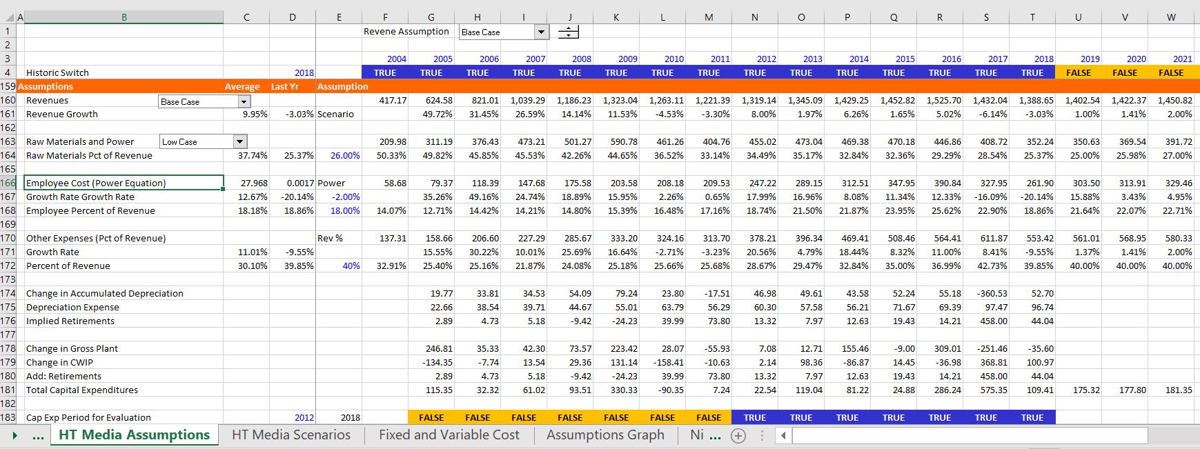
The manner in which assumptions can be developed is illustrated in the screenshots below. The first step is using AVERAGEIF and/or LOOKUP to put in the average of the various assumptions over the entire historic period or for the last historic year. In the case of revenues, I begin by entering the revenues shown on line 160. This just comes from the historic income statement at first. You can begin with an if statement — IF(Historic Switch, Revenues). Note I have not yet implemented the forecast. The revenue growth is entered just below the revenues. For the historic period, the growth rate is computed simply as the revenues divided by the prior year revenues -1. Now it gets a little tricky. You can compute the average growth rate over the period by using the AVERAGEIF(Historic Switch Line, TRUE, Growth Rate Line). You can compute the growth rate for the last historic year using LOOKUP(Last Historic Year, Year Line, Growth Rate Line). If you lock in the historic switch line, the last historic year and the year line in the formulas, you can copy the formula to other assumption rows like the COGS divided by the revenues. Then you can see what the average and recent statistics are for things like COGS to revenues, depreciation rates, tax rates, growth in operating expenses, interest rates and so forth. Given these and other statistics, we can move to implementation of the assumptions in the forecast.

Different methods of assumptions calculations
Method 1: Using Fixed Scalars
In the example that I am using on this page I have included four different methods for establishing assumptions. The first method is a simple one where you just put in one scalar number. In the screenshot above these scalars have a blue colour because they are inputs. Other alternatives are to use a time series of different numbers (that can come from a scenario page). A third alternative is to use some kind of equation for fixed and variable cost. Each of these three methods is discussed below. The first method of using a single number is illustrated in the screenshot below. In the example, you enter a number adjacent to the average and recent statistics and this number is used in the forecast. For this example, I have used the accounts receivable (debtors) to sales. In the formula, you refer to the historic switch again and then, when the historic switch is false, you use the input number. The formula is: IF(Historic Switch, Debtors/Revenues, Fixed Number).
Method 2 – Time Series, Interpolate and Scenarios
The second method uses a time series of different values that change over time. In entering time series assumptions, you should probably add a separate sheet. To illustrate this technique of working with time series assumptions, I present two screenshots below. In the first screenshot below, I show how you may set-up different growth rate scenarios in a separate. I have added a sheet and plopped in a couple of scenarios. As usual, you begin with a scenario number and then create a table with the INDEX function. With results from the INDEX function and maybe a drop down box or a spinner box, you can create a time series for use in the model. Next, you can use the interpolate function as described in another web page, to lay out the year by year numbers. An example of such a scenario page with time series data that changes over time is illustrated below.
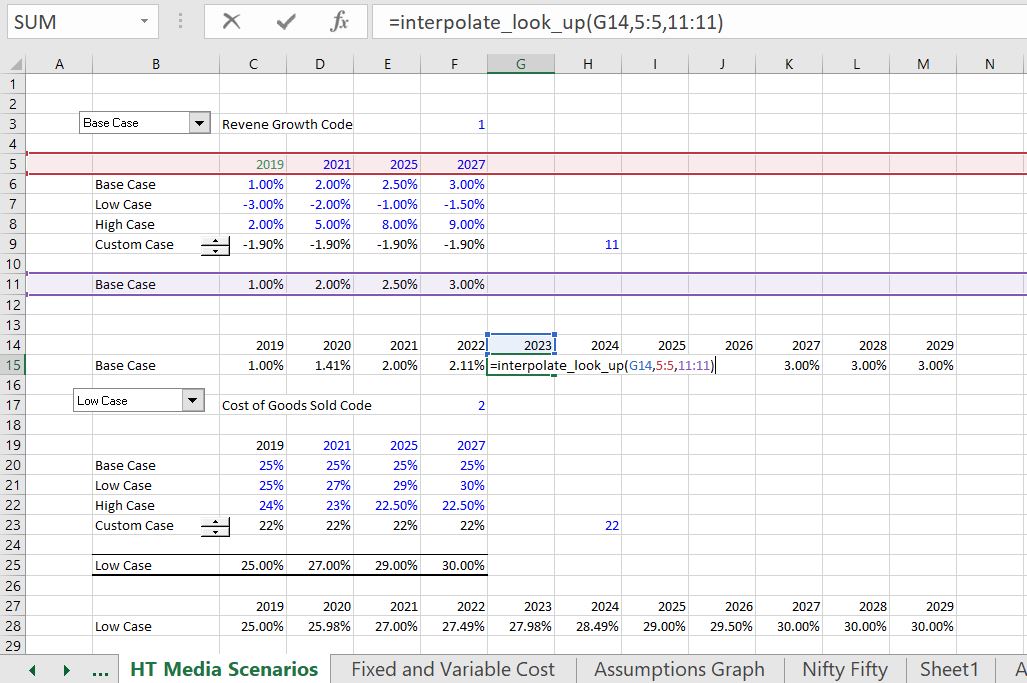
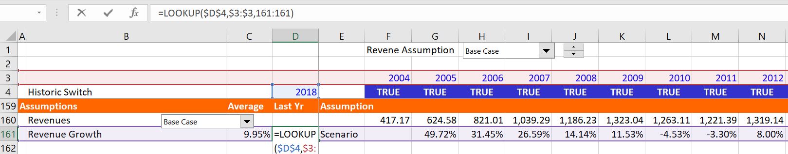
Once you have defined a scenario with a time series as shown in lines 15 and 28 above, you can use the LOOKUP function in the assumptions section instead of the simpler fixed number that was explained above. This formula is illustrated in the screenshot below for the case of revenue growth that comes from line 15. I have used the colouring function from the generic macros (see the link) and selected the green option. The formula is too long for me, but this may be an exception to the rule of very short formulas.
Method 3 – Evaluating Fixed and Variable Costs with Scatter Plots
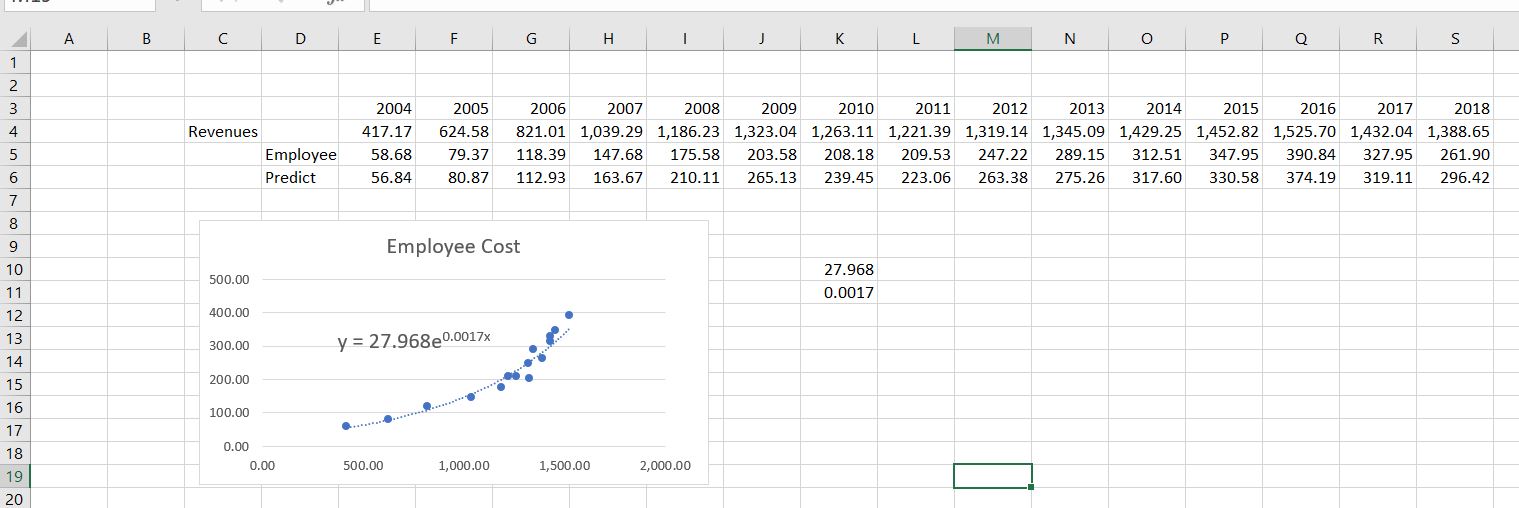
In making assumptions for corporations, you would like to know what costs are fixed and what costs are variable. If most costs are fixed and do not change with revenues, the cash flow in upside cases will grow fast, but in the downside cases when revenue falls and the fixed costs remain, the pain will be worse (this is what happened in a sense to U.S. automakers after 2008). To investigate whether costs are fixed or variable, you can try and make a scatter plot that is illustrated in the screenshot below. To make the scatter plot, make sure the x-axis, or revenues, does not have a title. Then you can try to add different trend lines. If costs are fixed, there should be a positive intercept at the x-axis (if you did this really carefully, you would deflate the expenses). As with the revenue scenarios, I put this into a separate page. For the case shown below, a exponential function seemed to fit best. Then you can implement the function in your assumption. Note also that I have verified the formula in line 6 that is called predict. Here, the expenses are computed as 27.968 * exp(revenues * .0017).
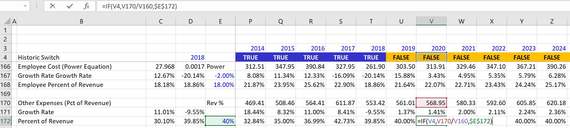
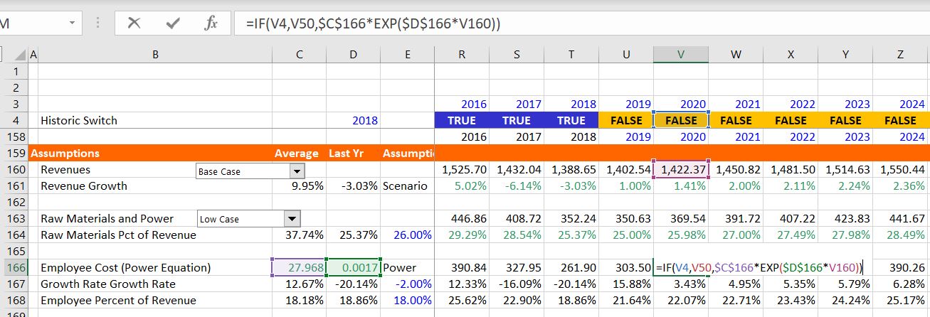
Once you have a formula that defines the cost as a function of revenues, you can implement the formula into your forecast, whether the formula is a linear equation, a polynominal equation or a power equation. Before you implement your forecast you can assure that the equation is resulting in a reasonable forecast as shown in line 5 of the above screenshot. This time when you enter the assumption, you can put the equation into the assumption equation and use the historic switch as usual. For the expense forecast implementing the equation is illustrated in the screenshot below. The formula has the following form: Expense = IF(Historic Switch, Actual Amount, 27.69 * EXP(Revenue * .00017).
Presenting Key Assumptions with Flexible Graph and Historic Switch
In assessing the assumptions I suggest you make a graph using the INDEX function to make flexible graphs with a spinner box as explained in the associated link. As in other cases where you want to take numbers from a sheet with a bunch of stuff, you can begin with a row number. As usual, after the row number, use the INDEX function with an entire column. Then add a spinner box and/or a combo box to the row number, blah, blah, blah. The difference in this case is that you should put in the historic switch so that the historic values will be different from the forecast values. You can also use the trick where if the forecast has no values, i.e. the line is blank for the forecast, then you do not want to show the line. To do this you can go to the page for spinner skip which is linked to this sentence and then copy and paste the macro. When you are finished, the graph of assumptions and forecast may look something like the screenshot below.
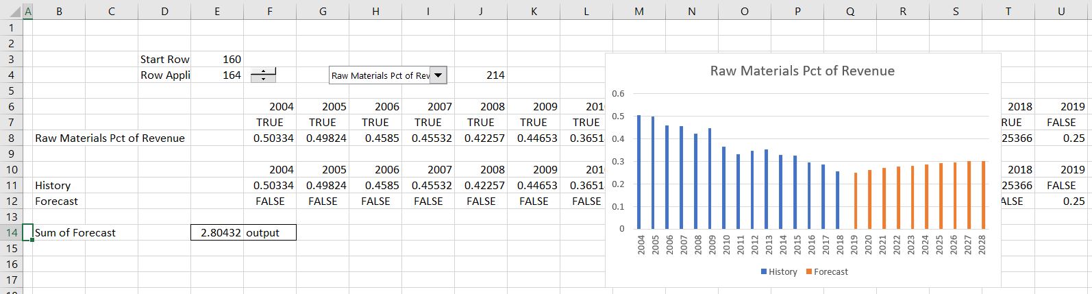
I hope that you do not muck up your model with a bunch of different scenarios. Instead you should put the scenarios for key variables like sales growth, margin and capital expenditures in a separate page. The screenshot below illustrates how you could put some of the assumptions with the history and forecast in a graph.
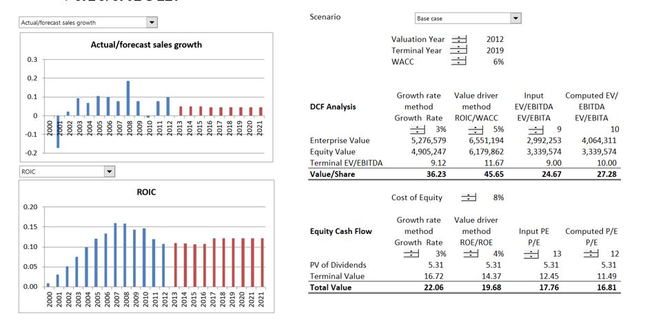
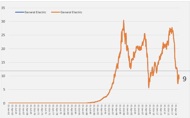
The screenshot below illustrates the idea of presenting history next to assumptions. It is from Value Line and I remember using these summaries in the 1970’s. But the idea of showing all of the long-term history and evaluating the ROE and ROI in the forecast as a test of the assumptions is still very attractive even with all of the stuff you can find on the internet. In the case a hand, the ROE forecast for GE was 15% and the projected stock price from EPS x P/E ratio was projected to range from 50 to 35 with an average 42.5. The actual price
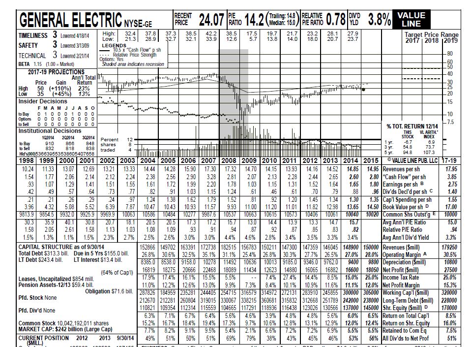
Note that I am not saying the forecasts are good. Because of questionable acquisitions (Alstrom) and a big decline in the demand for turbines after renewable energy, the projected price per share shown on the top left did not materialize. The high price was supposed to be 50 and the low 35. As shown below, the actual price was 9 in 2019.