For most projects, investments do not have the same life and some capital expenditures are often required before the end of the life of a project. When accounting for projects with different lives, you can put in replacement cost with inflation and with learning, but unless the life of the replacement is the same as the divisible by the life of your project, you will have a problem. If you use the method I suggest for computing levelised cost you can compute a series of different project components. For example, in the case of batteries, the life of the battery will surely be different from the life of a solar panel and how can you compute the cost of both the battery and the panel in an integrated model if the life of a battery is 20 years and the solar project has a life of 30 years. On this page I demonstrate how the LCOE addresses this issue and the more tricky issue of what happens where there is a learning rate and the replacement cost is lower than the original cost in real terms. For example, what is the overall levelised cost when the cost of the second battery replacement is a lot smaller than the initial battery.
The problem with different equipment lives is important in the analysis of hydrogen where the lifetime of the stack in an electrolyzer is different from the other equipment and the lifetime of a truck is different from the lifetime of compression and storage equipment. The file below includes various different examples where I demonstrate how you can efficiently evaluate different replacement timing and even incorporate the differences into a financial model.
.
.
Introduction — Two Methods of Accounting for Replacement Cost with a Simple Example of Divisible Life
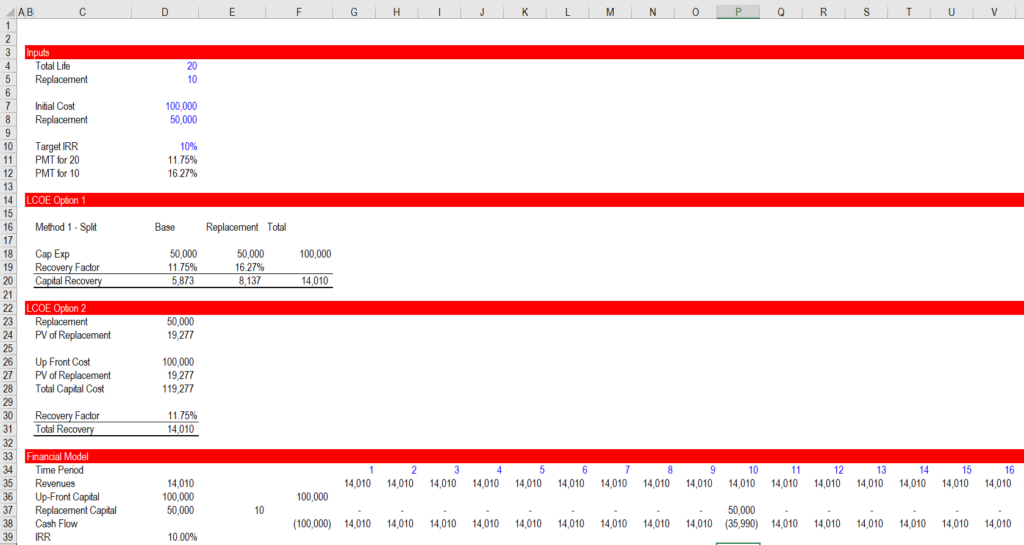
The screenshot below illustrates the case without inflation where the bases cost of a project is 100,000 and the replacement cost is 50,000. The overall life of the project is 20 years and the date of the replacement is in year 10. To solve this problem you can use two alternative calculation methods as described below. Note that you cannot solve this problem with the method 2 without considering residual value if the replacement period is not divisible by the overall life without a remainder (e.g. 20 divided by 8 would not work).
Method 1 – Split the Project into two parts
- Split the capital expenditures into the portion that will be replaced and the portion that will not be replaced
- Use a shorter carrying charge for the portion that will be replaced and has a shorter life
- Combine the carrying charges for the two parts.
Method 2 – Compute the PV of the Replacements
- Compute the PV of the replacement using a simple PV calculation (replacement cost/(1+discount rate)^replacement period
- Add the PV of the replacement to the base capital cost (the entire 100,000) and use this as the capital cost
- Apply the PMT function with the entire life of 20 years to the capital expenditure including the PV of the replacement cost
In the screenshot below I demonstrate that if the cost of the replacement does not change, that you can measure the LCOE using the shorter life using either of the two methods and you get the same financial results (i.e. the IRR) as if you would make the replacement. As usual, you should test the method with a financial model.
.
.
Replacement Cost with Taxes
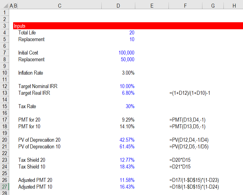
In the prior webpage I describe you can account for tax effects in two steps. The first step is dividing the PMT formula by (1-t) to account for taxes that will be paid on equity. The second step is to compute the value of the tax shield as a percent from the PV of the tax depreciation at the pre-tax rate multiplied by the tax rate. The fundamental calculations are illustrated in the screenshot below with the PV and PMT formulas. Note that if you use accelerated depreciation the calculation is a little more difficult. I show a UDF to resolve this issue in the accompanying web page that works through taxes.
.
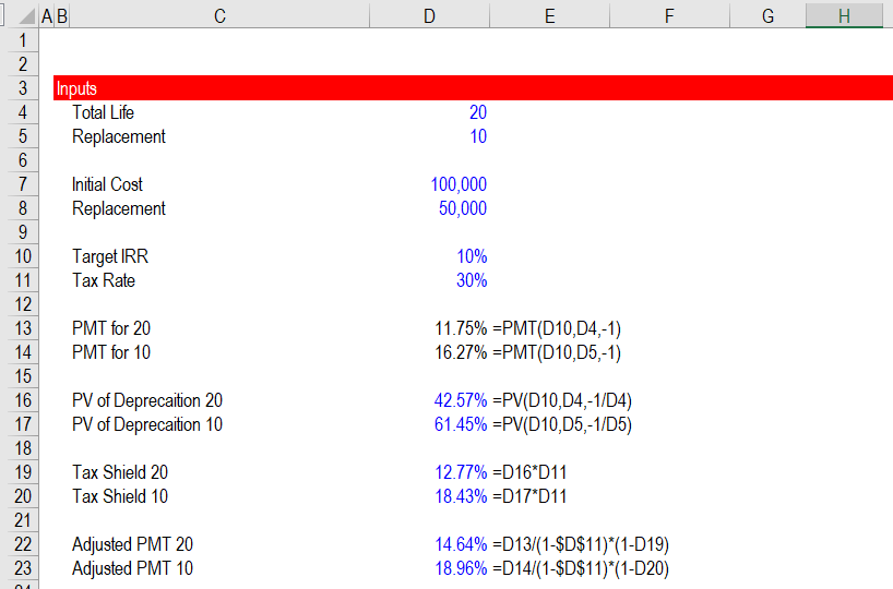
.
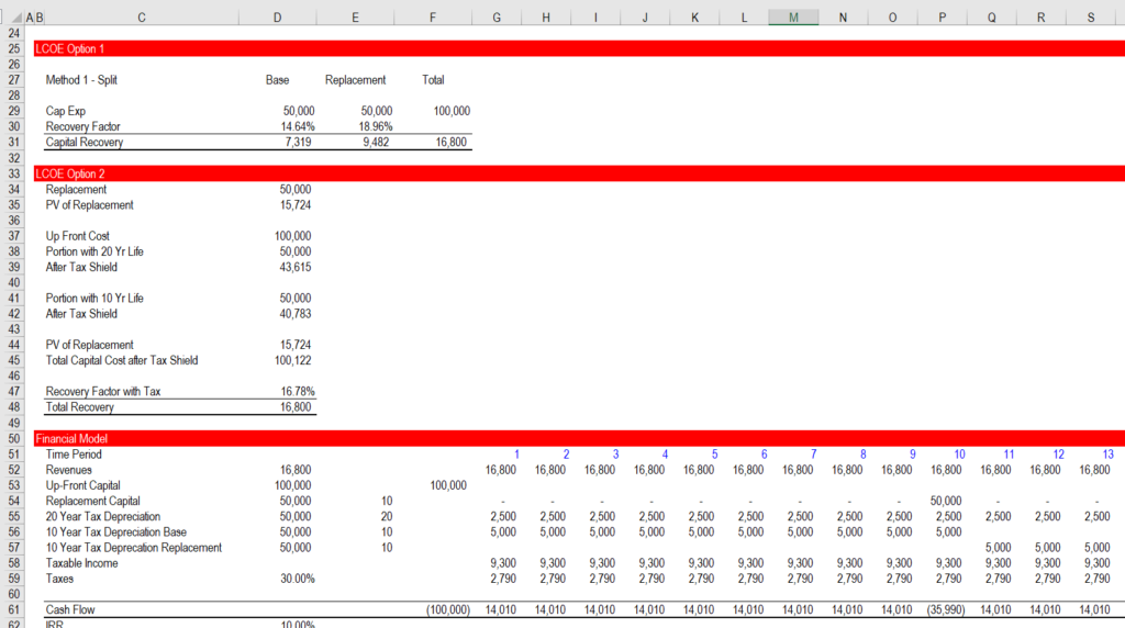
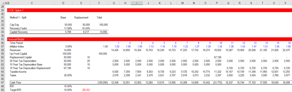
Once you have made the adjustments in the PMT calculations, you can verify the calculations with a financial model. However, this verification is becoming a bit more difficult as you must array the tax depreciation with the timing of the replacement and include alternative depreciation calculations. Note in the screenshot below that there are three different depreciation lines:
- First, for the base asset that is depreciated over the entire life
- Second, for the first part of the cost that is split into the replacement
- Third, for the second part of the depreciation on the replacement with the shorter life
.
.
If you include inflation, it is simple if you set-up your model with two columns. You could set up the model as illustrated below if you are using real costs. You can look at the formulas, and use the real IRR in the PMT formulas. Note that the PV of the depreciation is computed at the nominal and not the real rate.
.
Once you compute the real carrying charge rate, you can put things into the financial model with an inflation index. Note in the screenshot below that replacement cost is inflated and the associated depreciation is inflated. Once the inflation is included, note that the IRR is the nominal IRR is obtained. As with other discussion of the real IRR, note how the revenues are inflated and the 10% target nominal IRR is achieved.
.
.
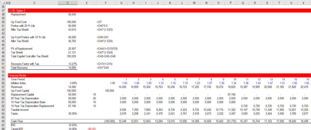
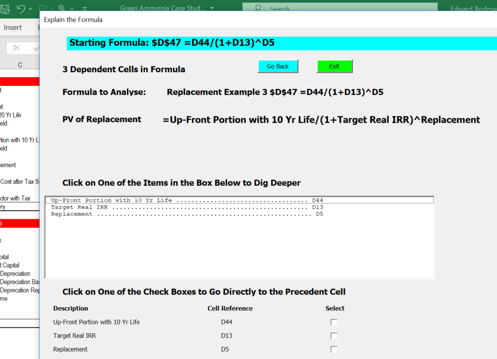
If you use the second method and explicitly consider the dates and the NPV of the replacements, you can arrive at the same number. But you have to be careful about computing the NPV of the replacement and then separately adding that to the carrying charges. The method of directly incorporating the NPV of the replacement into the carrying charge is illustrated in yet another screenshot below.
Note the formula for the PV of Replacement that is:
Replacement cost/(1+real rate)^10
This is multiplied by the tax shield
.
Replacement Cost when the Project Life is not Divisible by the Project Life with No Remainder
For me, the biggest reason to use the two column method for replacement cost is when the project life is not divisible by the replacement period. For example, say the replacement occurs in year 15 in our 20 year example. I note that there is an even more powerful argument for the column method if the replacement cost multiple times. In this case, you can make three arguments about what could happen:
- There could be a residual value where you would sell the asset (such as a battery or the stack portion of an electrolyzer or an inverter.
- You could buy a used piece of equipment with a life that has the expected life of the replacement part.
- You could assume that the entire project retires early
- You could assume that you replace the equipment and then you throw it away
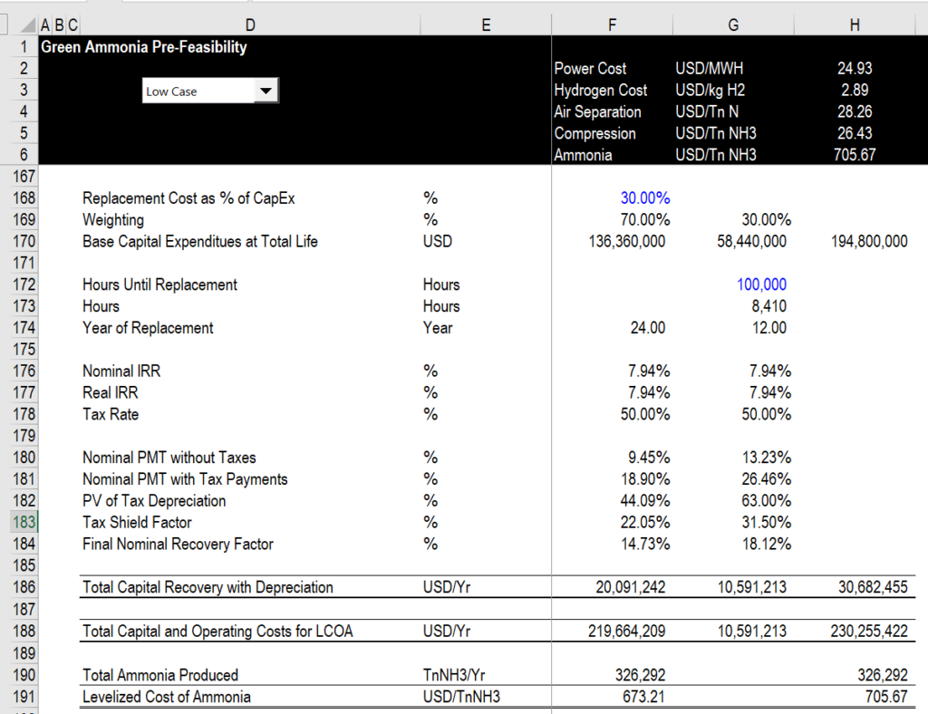
Replacement Cost with Learning
When you include learning you can give credit to the LCOE for the expected lower cost of replacement. You cannot simply use the average of the replacement cost because the replacement cost of the replacement cost has a lower value. To do this you can determine the weighted average cost of replacement with the lower future replacement. To get to the weighted average you can compute the
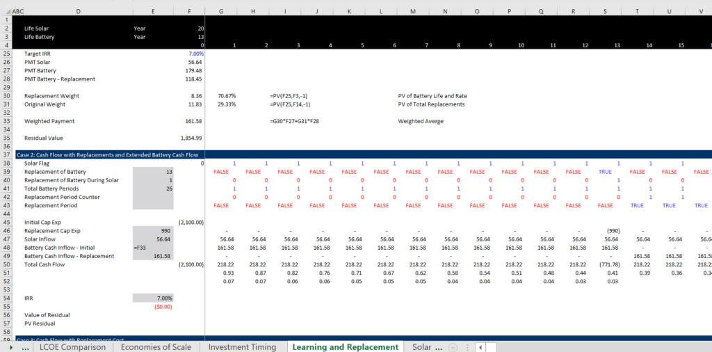
The screenshot below illustrates the effect of the learning.
Comparison of Using the Method of Separating Assets with the Method of Computing the PV of Separate Replacements
In this section I demonstrate two different ways you can compute the effect of replacements on levelised cost of something. I argue that it is far easier for you to separate the assets into two columns. But if you insist on computing the financial model with residual values and learning rates, you should understand and use the second method were the individual replacements are computed and then can be imported into the financial model.
The approach to using two columns for replacement is illustrated below. Note that the replacement is computed using a different lives.