Waterfall Chart Templates (Excel 2010 and 2013)

This page demonstrates how to use a template for creating a waterfall graph that walks through changes in one variable to another. You can quickly format a group of data that has a starting point and an ending point and demonstrate how to get the start to the end.  The waterfall graph is created from a macro that can be implemented by only having the waterfall file below open.

This is a sad page for me. I spent a lot of time making what I though was a really flexible program to make waterfall graphs. The waterfall graph program works a little like the read pdf file and the generic macros file. You just open the file named waterfall graphs and then, as long as your data is formatted correctly, you can make a variety of really flexible waterfall charts. After I finished what I though was a really cool new version of the waterfall graphs I found out that excel 2016 added these charts to the normal repetoir. That was so sad for me. But if you have earlier versions of excel and you want to put in waterfall charts, I think this page can be really helpful to you. The file that you can open and then press SHIFT, CNTL, V if you have excel 2013 or later is available for download below.

Excel File with Waterfall Macro That You Can Implement By Pressing SHIFT, CNTL, V After You Have Formatted Your Data

 

If you are old-school and have excel 2010, you can follow the same process whereby you open the file and then press SHIFT, CNTL, V.  Again, you open the file and then go back to your file.  In your file you select the data area described below and then, in your file (and not in the waterfall file), you press SHIFT, CNTL V.

 

Excel File with Waterfall Macro That Works with Excel 2010 and is Implemented By Pressing SHIFT, CNTL, V

This page documents a WATERFALL GRAPH file that I have created that accepts data and automatically creates a WATERFALL GRAPH. You can make a WATERFALL chart within seconds and the waterfall graph will change when you change the inputs. After opening the file named “WATERFALL CHARTS.XLSM” you go back to your file with data. There should be a note on the status bar of excel file (the bar at the bottom of the file) that states “Press SHIFT, CNTL, V to Make the Waterfall Chart”. When you are back in your file select two adjacent columns, the first has titles, the second has data. The data should begin with a base case value and then have incremental additions or reductions to the base. The last row that is selected should have a title and no data. You then press the SHIFT, CNTL, V and a waterfall chart should be made. In order for the waterfall chart to be structured, the macro puts data into a new sheet in your workbook that can be hidden.

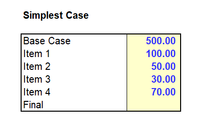
Step by step instructions for operating the file are included below with screenshots.  The first step is to open the waterfall file so the maco will work. After opening the file, you should the note SHIFT, CNTL, V in the status bar of excel at the bottom of the file.  Then, go back to your file and format your data. If you do not have any subtotals the screenshot below demonstrates how to set-up the data.  You need a base amount, then below the base data some increments and then a space for the final bar at the bottom.

 

 

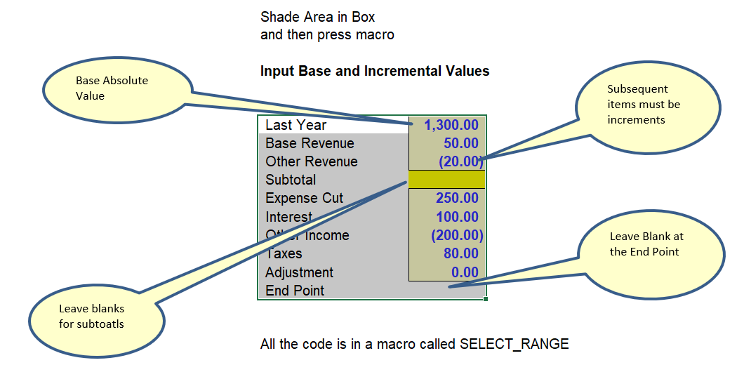
A somewhat more complex case is shown in the screenshot below with some comments.  This case has some negative numbers and some spaces for subtotals.  When you have a subtotal, there will be a separate blue line.  Once you have data in this format, select the data and the titles and then press SHIFT, CNTL, V.

 

 

 

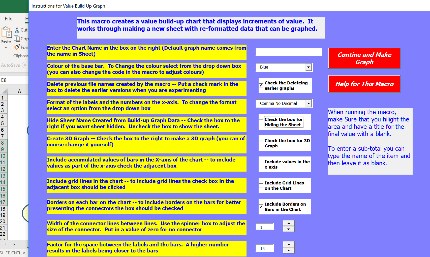
After selecting the area and pressing SHIFT, CNTL, V you should see a user form with a bunch of questions.  I suggest leaving the defaults and just clicking on the box that is titled Continue and Make Graph.

 

 

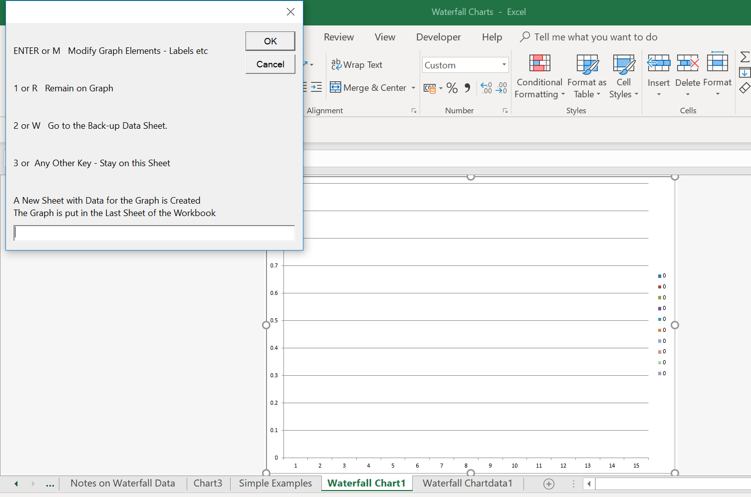
After pressing the red Continue and Create Graph Button, an input box that asks a question that is shown below. If you have excel 2016, just press ENTER.  Then a second screenshot appears as shown in the second screenshot below.  Again, you can just press ENTER.  After that, a waterfall graph should appear.

 

 

 

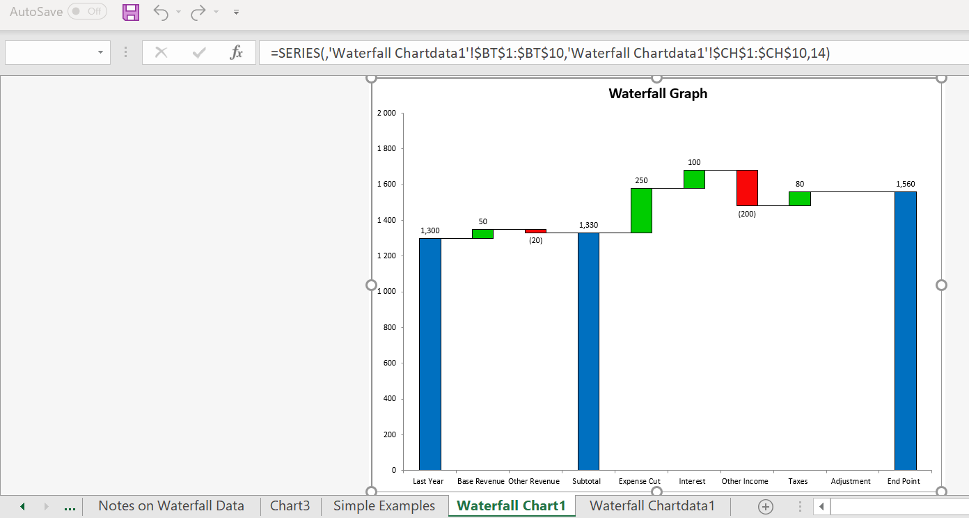
After pressing ENTER for these two Input Boxes, you a waterfall graph should appear in your file.  In the example above, this graph is shown below. If you see this graph you should be impressed by the little straight lines and the numbers above and below the bars.  These were a real pain to make.  That’s why I am so depressed about the graphs in excel.

 

 

 

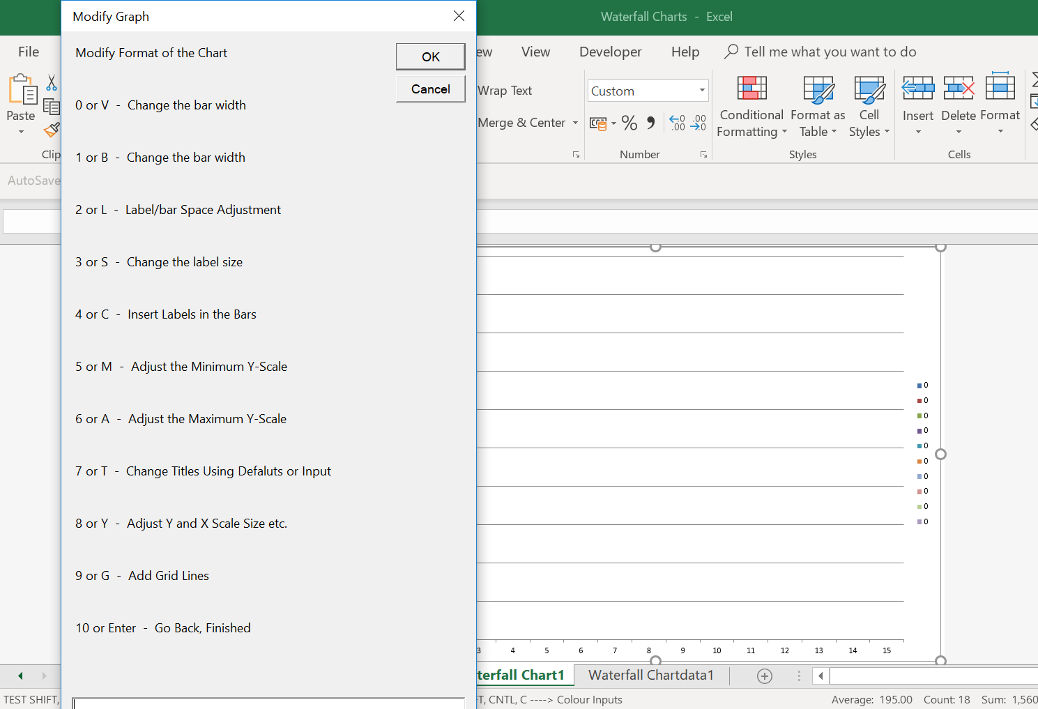
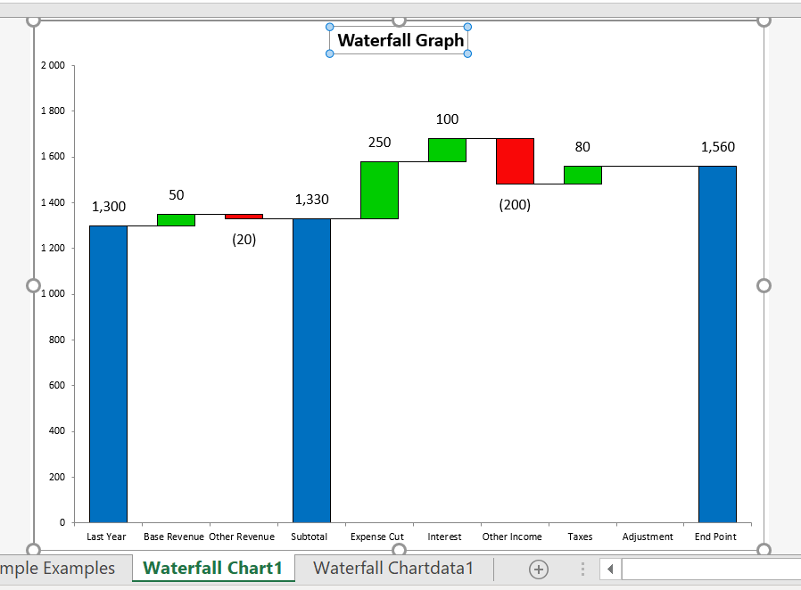
Finally, I spent a lot of time on making the graph flexible.  You can do this by pressing SHIFT, CNTL, E.  Then you have options to make the bars wider or thinner.  You can make the labels bigger or smaller.  You can change where the labels appear …..  In the screenshot below I have made wider bars from pressing SHIFT, CNTL, E and then I have also changed the size and placement of the labels.

 

 

 

Your file is not messed up with macros as the waterfall chart macro works from a separate file and creates a sheet that arranges data. You can use the technique to build multiple waterfall charts. The videos below give you a guide as to how simple this process is. The waterfall chart videos are all quite short, reflecting the fact that the process of using this technique works quickly.

 

Videos for Quickly Creating Waterfall Charts

 

 

 

 

 

 

 

 

 

 

 

 

 

Files on Resource Library that You Can Access by Sending an E-mail

Some of the files in the scenario folder that may help you include: