This page introduces cost of capital issues using the now very standard capital asset pricing model. Coming up with a cost of capital number can be frustrating from both a theoretical and a practical data standpoint. This is particular the case with CAPM where the estimate depends on parameters that are impossible to measure (EMRP) or are not stable (Beta) or are mis-characterized (Rf). In this page I demonstrate how easy it is to compute beta; how the beta can be unstable over time; the relationship between beta and volatility; how mean reversion adjustments to beta are crazy; how size adjustments to the cost of capital come from nowhere; and absurd attempts do compute the unlevered beta and then re-gear the beta.
This is before explaining that a 10-year treasury bond typically used to represent the risk free rate is not close to risk free because investors take inflation risk and before I go a bit crazy by discussing how crazy the measurements are for the equity market risk premium. The main reason I have made this page is to provide a basis for studying other methods (which also have problems). To introduce some of the cost of capital issues that I evaluate in subsequent pages, I have included a set of power point slides that evaluates alternative methods for renewable projects.
For many issues associated with the cost of capital it is deceptive to assert that there is any real science to the estimates and to pretend that there are not many unresolved issues in the theory and the data used to estimate the cost of capital. The CAPM is commonly used for estimating the cost of capital, but inputs for the model are subjective and the model has theoretical problems. The CAPM is difficult to implement and problematic not because of some academic study that questions whether beta is the only relevant measure of risk. The real problems with the CAPM comes about because of difficulties in measuring the risk-free rate, the beta and most of all the equity market premium. As there are many theoretical and statistical issues with each of these variables, the only real alternative to the CAPM is deriving the cost of capital from stock values and the expected cash flows.
Comments: Well, last year I took Damodaran’s class. I started to butt heads with him, because so much of the class was spent on CAPM, and I just don’t believe in CAPM. I don’t believe in beta, and I don’t really believe that we should judge WACC based of market equity instead of book equity. (NFLX, BA, HD, just to name a few, REALLY show the failure of WACC) Anyway, after that class I came across your site and I’ve been digesting all your material. Which I want to stop and say THANK YOU!!! You’re material is the best I’ve seen anywhere in all my days of doing this, online, 100-200 finance books read, etc.
.
.
Power Point Slides Evaluating Alternative Cost of Capital Methods in the Context of Renewable Energy
The most basic problem with estimation of the cost of capital is that nobody can observe the number. There are no contracts between investors and a company that write down the percentage cost of equity number such as 12.5% for the cost of equity capital; you cannot track cost of capital changes in the same way that you can see changes in stock prices, interest rates, gold prices, exchange rates and other things. These days you can easily find data for things like earnings per share, operating income, cash flow, price to earnings ratios and so forth for companies on the internet; but you cannot find a number for the cost of equity anywhere. Furthermore, measuring the cost of equity is different from measuring the cost of debt. Components of the cost of debt are written in loan contracts where parts of the interest rate such as the base interest rate and the credit spread are explicitly written down in loan agreements. These credit spreads are collected in databases.
As the cost of equity cannot be directly observed, different methods have been created to implicitly derive and estimate the cost of equity. But all of the methods require estimation of variables that are subjective. These subjective variables include the market risk premium; the beta; the expected growth rate; the expected return, and the expected market risk premium. This difficulty in measuring the cost of capital should be a backdrop for all of the seemingly sophisticated economic equations that are used for variables like beta, country risk premia, expected growth rates and other items.
Given the difficulty in measuring the cost of capital, I begin with a definition of the cost of capital, which is not as simple as one may think. The cost of capital is not simply the rate of return that is desired by an investor. Rather, it is the minimum return that is acceptable for to compensate for taking risk. The key word here is minimum. It is not the expected return; it is not the return that other people get on investments. For example, when an investor complains that the rate of return is too low to invest in a hydro plant, the investor is correctly interpreting the meaning of the cost of equity. But if the investor would continue build the hydro plant even if the return was lower, this return for which the investor would not walk away is not equal to the cost of capital as defined by the minimum acceptable return.
You can think of the cost of capital in a bidding context. In a highly competitive bid for a project that does not have some kind of provisions that give one company an advantage over another company (e.g., a solar plant bid in Dubai). You want to win a bid and offer a low price. Your manager wants a pretty high return. If you are to have any chance of winning the bid, you negotiate with you manager to push down the acceptable return to win the bid until you arrive at the minimum acceptable return. This minimum return must compensate for the risk you take if you win the bid. You can imagine how difficult it is to come up with a true number.
Introduction: Problems with CAPM as a Basis for Estimating the Cost of Capital
1. Rf — how can the long term T-Bill with inflation risk be risk free. I would be terrified about risk of changing inflation for bonds and I think this is a bigger risk than investing a stable old food or beer company or a utility company.
2. Beta — you get completely different betas when you use daily or weekly or monthly data which is extremely simple to get from Yahoo. Then the silly people put in the mean reversion which comes from a horrible paper written in the 1970’s that had no proofs at all.
3. EMRP. When you make very simple compound growth rate computations about real returns or returns in markets the whole EMRP is nowhere near the 5.6% of Damodoran. This is a very big problem.
4. Adjustments — adjustments for country risk, small company risk, liquidity risk are the worst of all. How can people possible believe this magic potion that has no basis in theory and comes from completely black box stuff.
Price per share = EPS * (1-g/ROE)/(k-g)
EPS = ROE * Book Value
so
Price per share = ROE * Book Value * (1-g/ROE)/(k-g)
(k-g) * Price per share = ROE * Book Value * (1-g/ROE)
k-g = ROE * Book/Price * (1-g/ROE)
k = ROE * (1/PB) * (1-g/ROE) -g
This k depends on ROE and Growth Rather than Beta, Rf, Adjustments, EMRP but at least it is an alternative and for many companies the ROE is pretty constant. I am trying to work more on this as well as getting the k from the P/E ratio.
I believe that cost of capital and the CAPM is a silly idea that has taken off and makes no real sense. It seems to conform to what people want to believe — a simple model from a magic potion. The CAPM is a lot like the story of people buying marijauana with food stamps. It is untrue, but it gets a lot of press.
Estimation of the cost of capital cannot be avoided in valuation (directly or indirectly) and many people are still proud of themselves by applying the CAPM where comparison companies unlevered Beta is computed and then translated into the weighted average cost of capital. These days, cost of capital estimation is debated and people seem to apply the CAPM without really believing it. One of the quotes from Taleb that I like a lot is when he compares believing the CAPM to believing that a magic potion sold on the internet will cure your sickness.
Many analysts know that the CAPM model has never been confirmed from an empirical standpoint and the model requires many subjective inputs including the equity risk premium and ridiculous adjustments to beta for mean reversion that came from poor analysis in a paper written in the 1970’s.
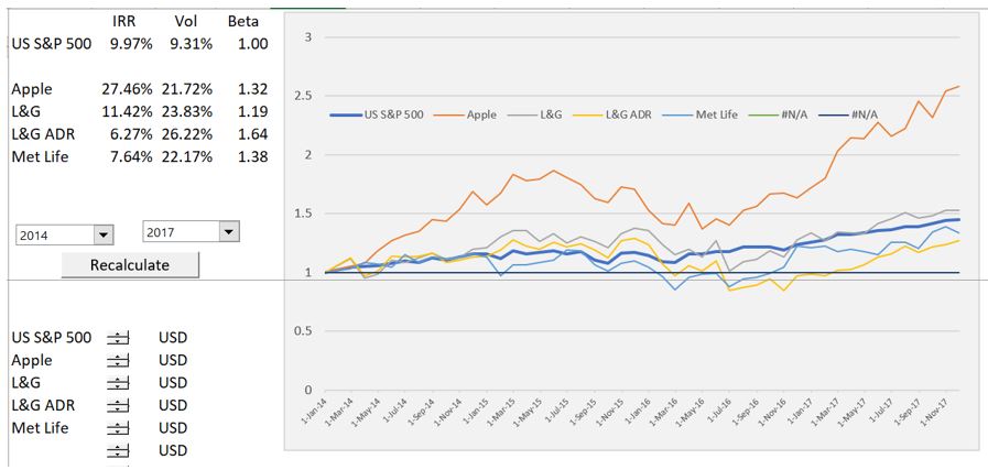
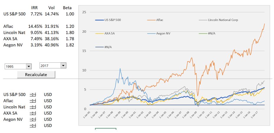
I introduce the CAPM by demonstrating how to work with stock price data that you can collect from finance.yahoo.com to compute beta and estimate the CAPM. I demonstrate how easy it is to compute beta and present data using scatter plots. The mechanics of computing beta are demonstrated and then problems with the stability of beta are documented using different cases. Using the scenario manager it I demonstrate that there is a high correlation between beta and volatility and the instability of beta.
After discussing beta, I turn to the question of the equity market risk premium. Some have suggested that the equity risk premium can be as high as 10% (which is totally crazy). I try to prompt you to think a little differently about the subject and use some stock price data to demonstrate a fundamental point. When the equity risk premium is higher than the zero, there will be a continual increase in the disparity of income between rich people who own stocks and poorer or middle class people who don’t own that many stocks. This does not answer what the equity risk premium should be, but it does demonstrate a fundamental dilemma with the theory. It even explains a pretty obvious point that a lot of the increase in the dispersion in income comes from real increases in stock prices.
Computing and Analysing Beta
A very long time ago when I went to university, computing beta seemed to be a bit of a mystery and studying things like whether beta is stable; is beta different when you use daily, weekly or monthly data; is beta correlated with returns (like it should be because higher risks come with higher returns); is there any evidence of beta mean reverting over time; is the beta correlated to volatility (meaning that the true measure of risk may be volatility and not beta); and was the beta different in periods of high volatility than calm markets.
Nowadays all of these issues can be evaluated by working a bit with spreadsheets and downloading stock price data from yahoo.com. No need to buy data from Ibbitson and Sigfield; no need for a statistical package; and certainly no need for all of those stupid calculus equations and mysterious tables. All you need to know is that you can compute the beta using the SLOPE function in excel and you can turn on and off different points with TRUE/FALSE switches. You can easily download the overall stock index and individual stock price data for may years and alternative time periods (daily, weekly, monthly). You can also very quickly rearrange the data using the LOOKUP function.
So, lets begin with downloading a few stocks by hand from finance.yahoo.com. I have used a few boring utility companies; a few banks; a few insurance companies; a few high tech companies; and some industrial and food companies. My list is below:
- Consolidated Edison
- Chase Bank
- Morgan Stanley
- L&G Insurance
- Aetna Insurance
- First Solar
- Paypal
- Microsoft
- Amazon
- Apple
- General Electric
To illustrate the process I use one company, Atena insurance, as an example. The file with the simple example is available for download below this paragraph. The reason I just use one company here is because I have another file that automates the whole process for may companies and puts them all together. Go to yahoo and download the company’s stock price into a CSV file. Then you can also download the S&P 500 index as a basis for computing the beta. You should use the adjusted prices for stock splits and dividends because these adjusted prices represent the returns realised by investors.
To compute beta, follow the simple steps below:
- Use the lookup function to put the S&P index next to the stock price. You can use the formula =LOOKUP(date for stock, entire column of dates for S&P 500, entire c0lumn of S&P index). This is illustrated in the screenshot below.
- Compute the return on the stock and the return on the S&P 500 after you have used the LOOKUP function. You can compute returns as the natural log of the current adjusted stock price divided by the previous period stock price. Computation of the returns is illustrated in a second screenshot. The formula is =LN(Current Price/Last Period Price). This is just like computing the growth rate — current/last – 1, but it is continual.
- The beta is defined using the formula Change in Stock Price = A + B x Change in Index. You can compute the beta in excel by simply using the slope function: =SLOPE(Change in Stock, Change in Index). You can also use the LINEST function, LINEST(Change in Stock, Change in Index, TRUE, TRUE). For this function you must press SHIFT, CNTL, ENTER. Both of the methods of computing the slope are demonstrated in the screenshot below.
- You can create a scatter plot of the change in stock prices for the company on the y-axis and changes in the stock index on the x-axis and show the beta and the R-squared on the graph. To do this, all you have to do is delete the title of the x-axis and use the F11 or the ALT and F1 key. Then the x-axis will be the change in the stock index. You must change the chart type and select the scatter type after pressing F11 or Alt and F1. Then you can add a trend line and from the trend line options select the option to show the equation and the R-squared. The resulting graph is shown on the screenshot below.
- The beta is normally computed using an arbitrary period of 60 months or five years (I know of no theory that suggests there is anything special at all about this period). If you want to compute the beta for different selected periods, you can enter a start and an end date. Then as with any date switch you can use the AND function and enter a true and false switch for the dates that are selected. The function is =AND(date>=start date, date<end date). Once you have the switch you can use an IF function with the switch and turn the unused data to FALSE. If the data is false, the slope does not use the date. Using the TRUE and FALSE is demonstrated in the screenshot below. In the second screenshot I demonstrate that the TRUE and FALSE method really does work using the SLOPE function and other statistical functions.
- You can also compute the volatility which is the standard deviation of the rate of change adjusted for the periods in a year. It uses the formula Standard deviation x Square Root (periods per year). It the data is annual, the volatility is the standard deviation. If the data is monthly, there are 12 months in a year and you use 12. If the data is daily, there are about 252 trading days in a year and you use that number. If there is no mean reversion the volatility should be the same whether different periods are used. Computation of volatility is illustrated in the screenshot below.
- Finally, you can compute the IRR. You can use the XIRR with the start and end dates or you can compute the growth rate using a CAGR formula. To establish the formula, you need to compute the number of days in the series and divide the days by 365.25 as shown below.
Is the Beta Stable over Time
To do this you can use the stock price database file. You can enter the stocks shown above and then change the periods to see what happens to the beta. To record the scenarios you can use the scenario manager.
Is Beta Different from Use of Daily, Weekly or Monthly Stock Price Data
The answer to this is yes. But it should not be if markets were efficient and had no mean reversion. To evaluate this issue, you can change the switch when you read the data. You may have to extend the periods and the files will be much larger and slower with daily data than for monthly data. Then you can do the same analysis with the scenario manager to record the different scenarios.
Is Beta Correlated with Returns
Beta should be correlated with higher returns because higher risks come with higher returns. You could do this for a gigantic database with hundreds or thousands of stocks. The analysis may be tricky because of beta changing. Maybe you could even take betas for a period and then compute the returns for a subsequent period.
Is there any Evidence of Beta Mean Reverting Over Time
Is the Beta Correlated to Volatility
If this is true that beta is correlated with volatility, this means that the true measure of risk may be volatility and not beta. This is a pretty easy study as the volatility is computed and so is the
Is the Beta Different in Periods of High Volatility than Calm Markets
To study this I compare 2007-2009 with subsequent periods. One could argue that the true measure of beta is what happened during the financial crisis. I have even written an article about this that you can download below.
Risk Free Rate
It is absurd to use the 10-year treasury to represent a risk free return because there is a whole lot of inflation risk in the 10-year treasury. By downloading the interest rate file, you can evaluate the historic difference between the yield on the 10-year and the short-term rate. It is clear that there is a premium for the long-term rate because of the uncertainty associated with inflation. This should be absurdly obvious but it is not generally applied.
Equity Market Risk Premium
Study of what happens when companies earn more than their cost of capital.
– Testimony on Cost of Capital and other financial issues (mergers, deferred taxes etc.)
Videos Associated with Valuation Concepts Lesson Set 1: Using Methods other than CAPM to Estimate the Cost of Capital
The set of videos for the cost of capital begins with an introduction to an approach that collects data from finance.yahoo.com and from marketwatch.com on stock prices, historic financial information, interest rates, earnings rates and growth rates. The database evaluates historic market to book ratios relative to projected return on equity to evaluate cost of capital. In addition PE ratios and published growth estimates are used along with assumed transition rates to back into the cost of capital. The CAPM is also computed along with the dividend discount model. The next set of videos explain the theory behind using the market to book ratio and the P/E ratio using simulation and sensitivity analysis. The final set of videos in the set explain details of how to build the data base.
| Cost of Capital Subject | File Reference | Video Link | ||
| Cost of Captial Database Introduction | Dow 30 Companies | https://www.youtube.com/watch?v=MOpSVBstv4o | ||
| Cost of Capital Sensitivity Analysis Using the P/E Ratio Formula | Price to Earnings Analysis | https://www.youtube.com/watch?v=A5FoWknb0HM | ||
| P/E Cost of Capital and Scenario Reporter | Scenario reporter | https://www.youtube.com/watch?v=j5DOUe6Wqbk | ||
| P/E ratio and Cost of Capital with Transition and Interpolation (Number 6) | Interpolate and Lookup | https://www.youtube.com/watch?v=XLVqKfvmjCM | ||
| P/B Regression Simulations for the Cost of Capital (Number 5) | Price to Book | https://www.youtube.com/watch?v=bhYlYSSWDVw | ||
| P/B Formulas and Cost of Capital | Price to Book | https://www.youtube.com/watch?v=s2NdJs8Su44 | ||
| Demonstration of Problems with CAPM | Beer Companies Database | https://www.youtube.com/watch?v=PL0zOQe-_6c | ||
| Collecting Data with Ticker Symbols | Cost of Captial Database | https://www.youtube.com/watch?v=MTskVI_VERk | ||
| Bulding Cost of Capital Data with Indirect Function | Cost of Captial Database | https://www.youtube.com/watch?v=UBl_pAvxhbs | ||
| Problems with Beta and Measuring Cost of Capital | Renewable Stock Price | https://www.youtube.com/watch?v=eTDjLjZo9cE | ||
| Use of Market P/E Ratio to Derive Cost of Capital | Economy Wide Cost of Capital | https://www.youtube.com/watch?v=GAolSYR1-pc | ||
| DCF Model | Integrated Electricity Model | https://www.youtube.com/watch?v=9rsxSVDbjxE | ||
| ……………………………………………………………………………………………………………………………. | … | ……………………………………………………………. | … | ………………………………………………………………………………………… |
Files Used in Advanced Valuation Concepts Lesson Set 1: Using Methods other than CAPM to Estimate the Cost of Capital
There are two general sets of files associated with the cost of capital analysis. The first set of files in the cost of capital set work through the theory of valuation and alternatives to the CAPM. The second set of files show how the models work with real market data. The set of files and videos below include both development of spreadsheets that measure the theory and explanation of how to construct comprehensive financial ratio databases that can be automatically uploaded to evaluate cost of capital. Deriving the cost of capital from the P/E ratio requires a lot of assumptions about long-term ROE versus cost of capital, long-term growth, inflation rates and transition periods. The P/E ratio files and videos use alternative scenario analyses to demonstrate the difficulty. The P/E Analysis file below evaluates the cost of capital with sensitivity and scenario analysis. It demonstrates how to correct the value driver formula P/E = (1-g/ROE)/(k-g) for inflation and changing returns.
- Price to Earnings Analysis.xlsm
- Cost of Capital and PE formula.xlsm
- Price to Book Analysis.xlsm
This files below evaluates the price to book ratio analysis with regression analysis and shows how to develop the formula: PB = (ROE-g)/(k-g). It shows how you can use the market to book ratio to compute cost of capital and it demonstrates how a regression equation for the market to book ratio can be used to evaluate the cost of capital. If the CAPM is a biased and flawed model, bizarre attempts to adjust the cost of capital for country risk resulting in premiums as much as 11% for some countries. These CAPM derived premiums published by a man named Mr. Damoradan and frequently used have to imply that the real cost of all sorts of products ranging from houses to electricity can be as much as double for so-called risky countries.
If you want to earn a badge for the cost of capital course, you first pick an industry, then you put your own ticker symbols into one of the three above files. Next, clear the existing sheets and re-run the macro to compute the cost of capital. Finally, send me the file with your industry and go through the various different methods to remove companies (with the TRUE/FALSE switch). Even though you will be doing me a favour by doing the painful job of finding the ticker symbols and entering them in a file, I will still charge 40 Euros for putting your name on the website. I will also post your file on this page and give you credit. According to modern marketing theory, you will feel much better about this process when you have to pay me money than if you did not have to pay. That is why I must charge a fee.