Depreciation on capital expenditues can be important in financial models for a variety of reasons even though depreciation is a non-cash expense. Reasons for modelling depreciation include computing taxes, evaluating operating income to compute rate of return, analysing the revenue requirements for companies that are regulated base on their cost of service where cost of service includes depreciation. The discussion begins with the theory of how depreciation relates to capital expenditures, gross plant and net plant with different growth rates. Given the theory on how depreciation rates stabalize, the next subject moves to more practical issues involving how to forecast depreciation in a corporate model where depreciation is separated between depreciation on new assets and depreciation on existing assets. When discussing depreciation for corporate models, calculating depreciation on existing assets is a big challenge. This is because information on when assets were constructed and when they will retire is not given (it is not reported in financial statements for example). Please note the straight line depreciation is used in this analysis.
In discussing how to compute depreciation in corporate models I begin by describing how to evaluate various relationships that can be derived by assuming that long-term growth is continual and the depreciation life is constant. This exercise is useful to understand various relationships (you can think about the average age of the population of a country with different growth rates and different life expentency). From a practical standpoint, if you are computing existing depreciation you can go backward and derive the historic growth rate in capital expenditures from the stable ratio analysis (this is like deriving the growth rate in the population from the average age of the population and the life expentency). You can go backwards which involves computing the ratio of accumulated depreciation to gross plant for many different combinations of plant life and growth rates. The ratio of accumulated depreciation to gross plant depends on these two inputs and is calculated below. The ratio and other ratios become stable in a long-term analysis:
- The stable ratio of capital expenditues to depreciation
- The stable ratio of depreciation to net plant
- The stable ratio of accumulated depreciation to gross plant
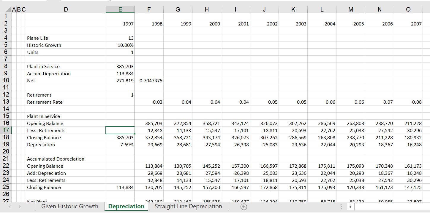
To begin depreciation analysis, the gross plant balance can be computed — this is the accumulation of capital expenditures less retirements. With the gross plant balance the depreciation expense can be computed as the gross plant divided by the depreciation life (gross plant depreciation rate is one divided by the life). Note that if the net plant is used for depreciation expense, the net plant depreciation rate is more complex and depends on the growth rate as well as plant life. Computing the balance of gross plant is the basis for evaluating depreciation that results from new capital expenditures as the new capital expenditures are simply accumulated and retire at the end of their life. The basic calculation of gross plant is illustrated below where it is assumed that the capital expenditures grow at a rate of 5% and the plant life is 5 years. The basic equations can be represented as:
- Gross Plant (t) = Gross Plant (t-1) + Capital Expenditures(t) – Retirements(t)
- Depreciation (t) = Gross Plant (t-1)/Plant Life
- Accumulated Depreciation (t) = Accumulated Depreciation (t-1) + Depreciation Exp (t) – Retirements (t)
- Net Plant(t) = Gross Plant(t) – Accumulated Depreciation(t)
- Depreciation Rate on Net Plant (t) = Depreciation Expense (t) / Net Plant (t-1)
- Capital Expenditures to Depreciation (t) = Capital Expenditures(t)/Depreciation Expense(t)
- Accumulated Depreciation to Gross (t) = Accumulated Depreciation (t) / Gross Plant (t)
The only equation that is a little tricky is the formula for retirements (this also the problem with existing depreciation as explained below). The key to computing retirements in excel is using the OFFSET function (which I do not like). When you use the OFFSET function, you should also use an IF statement that does not compute retirements when the period is less than or equal to the life. The general idea of this formula is:
Retirement = IF(period>=life,OFFSET(capital expenditure, zero row,-plant life))
.

.
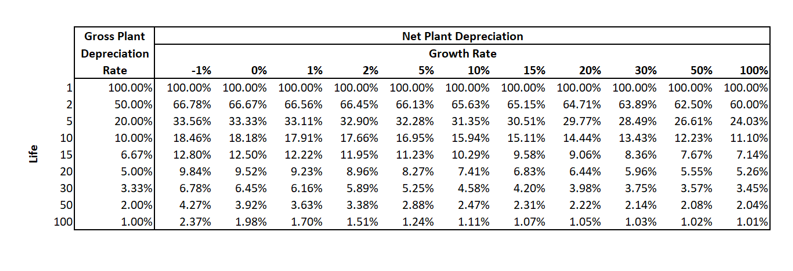
The table below shows the relation between plant life and the accumulated depreciation. You can see that the ratio is declining as the growh rate increases. You can also see that the ratio is higher as the plant life is longer.
.

.
.
When computing the depreciation rate in corporate models you can use the depreciation rate on net plant or gross plant. If you use the depreciation rate on gross plant you must consider retirements. If you use net depreciation rate you must be careful with changing growth rates. This web page demonstrates how to simulate retirements on existing assets so that you can model the depreciation on existing assets separately from new assets. The growth rate in retirements can be established from the accumulated depreciation and the base can be established from the amount of retirements necessary to make the balance of accumulated depreciation equal the gross plant by the end of plant life. To do this I set up a separate little page and then use the SOLVER function.
An effective way to deal with depreciation, is to first separate depreciation into depreciation related to new assets and existing assets. Depreciation on new assets can be computed using gross plant and reflecting retirements on the new assets. If the depreciation rate is not straight line, you can use a vintage depreciation function. The problem with existing depreciation is computing implied retirements. This can be accomplished by using the solver tool as shown in the videos and files below. The videos and files demonstrate how to make functions and the problems that can arise from incorrectly modelling depreciation.
The table below illustrates the net depreciation rate with different growth rates and different plant lives. note that when the growth rate is high, the net rate is closer to the gross rate. If the growth rate declines, then the net depreciation rate should also decline. With longer lived assets, the difference between the gross and the net rate is more extreme with age.
Step by Step Depreciation in Corporate Models from Gross Depreciation Rate
You can separate existing depreciation from new depreciation. Then, you can evaluate the retirements on existing depreciation using the process below.
The best way I have found to do this is to first find the historic growth rate in capital expenditures as well as a starting point for the retirements.
Use the Solver to Find the Base Level of Retirements and the Historic Growth Rate
To do this:
- Step 1: Derive the plant life for one category of assets or the assets in aggregate.
- Step 2: Set-up a schedule with gross plant that has balance from the balance sheet. Include retirements as part of the schedule.
- Step 3: Set-up a schedule with the accumulated depreciation that also includes retirements.
- Step 4: Put an equation with a base level of retirements and a growth rate to compute the amount of period by period retirements.
- Step 5: Use the Solver feature to derive the base level of retirements and the growth rate by setting the closing balance to zero.
- The way this works is shown in the screenshots below. The first screenshot demonstrates how you can set-up the balance of plant and the balance of accumulated depreciation. This balance is only for the existing plant.
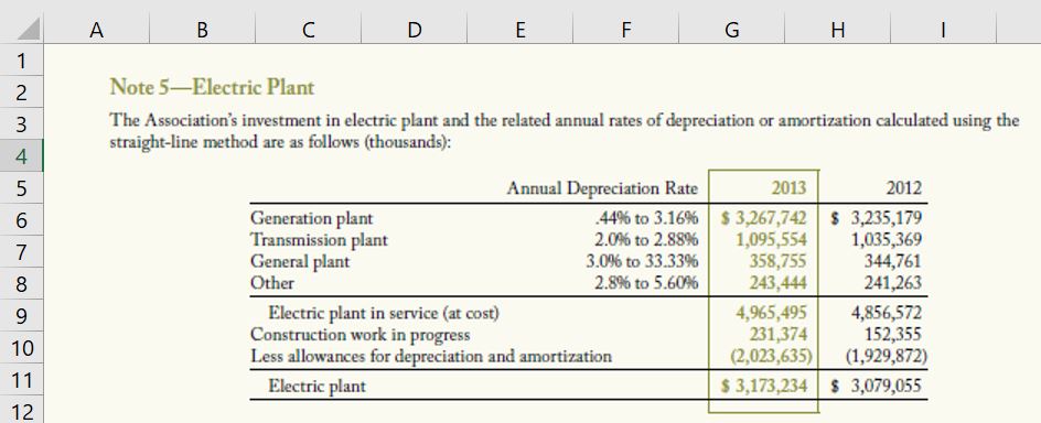
The second screenshot demonstrates where you can find information on the balance of plant and the balance of depreciation. With the balance of gross plant, you can divide the depreciation expense by the gross plant balance and derive the average depreciation rate as well as the plant life.
The next two screenshots illustrate how to set-up an equation for retirements. If the historic growth in capital expenditures has been constant, then the retirements should also grow at a constant rate associated with the existing plant. Of course this is a simplistic assumption and you could make some kind of other equation. The screenshot below illustrates how the base level of retirements as a percent of the gross plant provides the starting point for retirements. This is an arbitrary number that will result in the total amount of plant being retired.
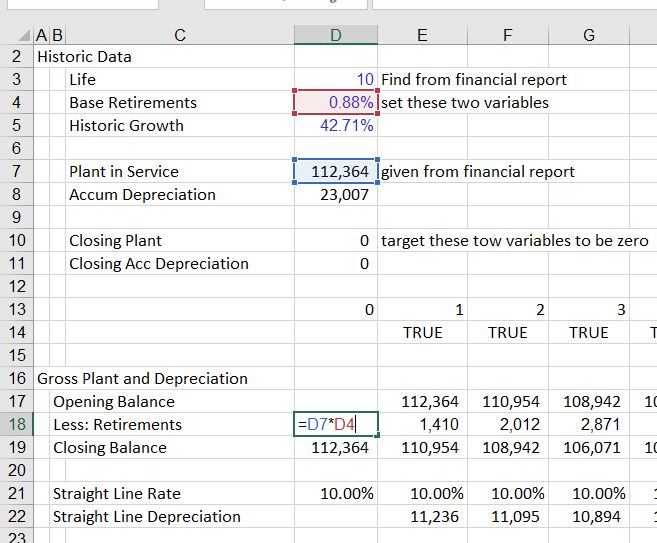
The screenshot below illustrates a few things. First, the screenshot illustrates how you can create the equation for retirements that grow over time. Second, the screenshot demonstrates that at the end of the life of the existing assets, the gross plant and the accumulated depreciation go down to zero. The task is to find the growth rate and the base level that results in the zero balances. The screenshot also illustrates how you can create a TRUE/FALSE switch that allows you to change the life of the plant. Note that you can make multiple classes of assets and compute the retirement amount for different classes.

The final screenshot illustrates how to use the Solver tool to compute the base retirement percentage and the growth rate. In the solver, the changing cells is both of the two inputs. The constraint is that the final balance of both the accumulated depreciation and the closing balance is zero. The closing balance is shown as a separate calculation in D10 and D11. The equations in these cells could use the Sumif function.

The file that contains an illustration of how to use the solver so you can find depreciation and retirements is available for downloading below.
Excel File with Depreciation Exercise that Includes Retirements and Changing Growth with Solver
User Defined Function for Finding Items in a Data Table
Function Table_Look_up(Lookup_Table, Lookup_Column, Table_Value)


Dim Index_Array(1000) As Double
Dim First_Column(1000) As Double
Dim Rows_in_Table As Single

test_index = WorksheetFunction.Index(Lookup_Table, 10, 4)

Rows_in_Table = Lookup_Table.Rows.Count

'
' First, compute the index
'

For i = 1 To Rows_in_Table

Index_Array(i) = WorksheetFunction.Index(Lookup_Table, i, Lookup_Column)
First_Column(i) = WorksheetFunction.Index(Lookup_Table, i, 1)

Next i

final_value = WorksheetFunction.XLookup(Table_Value, Index_Array, First_Column, 0, 1, -1)


Table_Look_up = final_value

End Function