This webpage discusses alternatives to the IRR. These alternatives include computing the risk premium earned on an investment and computing the return on capital from economic depreciation. The risk premium method involves first computing the ratio of the present value of the investment at the risk free rate to the initial capital of the investment. This defines the risk premium earned in terms of a ratio over the life of the project. This risk premium can then be spread out using different techniques. One technique is to simply levelisze the risk premium over the life of the project using the PMT function. A second method is to use a sculpting technique.
The other part of this page describes how to compute performance ratios using economic depreciation. This involves a couple of steps. First the value of the plant is computed using the project IRR. The difference in value from one period to the next period defines the economic depreciation. This is done at the original forecast for the financial model. Then the actual cash flow is used to compute the EBITDA and then the economic depreciation is subtracted. In this way, the economic performance can be evaluated for different periods.
Asset Management and Measuring Performance Using the Economic ROIC
This section describes how to apply performance management in asset management. An excel file with that illustrates the process is shown below.
.
.
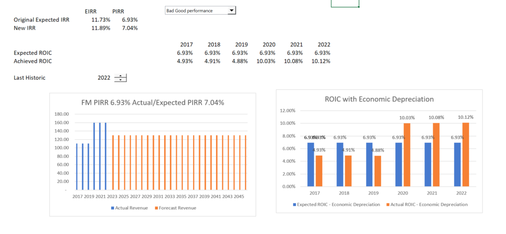
Results of the performance measure analysis is shown below. The revised IRR is shown in the screenshot below.
.
.
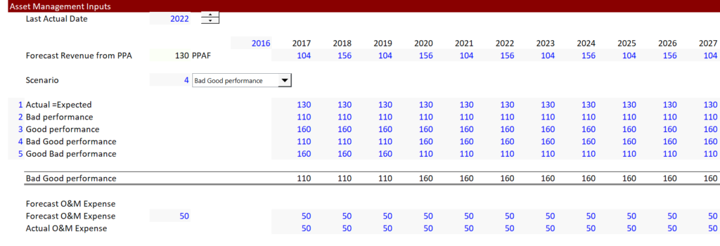
Inputs for the performance analysis is shown in the screenshot below. The screenshot shows that input includes the last actual year. In this way the actual can be compared with the forecast.
.
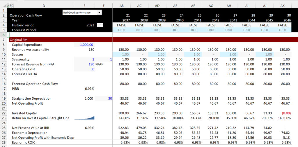
Mechanics of the asset management analysis are shown below. In the first screenshot the economic depreciation is computed and the economic ROIC is computed from the original financial model.
.
.
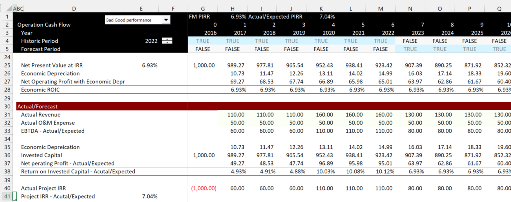
The next part of the mechanics of the analysis shows the actual and forecast. In this part of the model, the economic depreciation from the above section for the original FM is used. Note the low and then high ROIC computed.
.
Mechanics of Value to Investment Ratio
When computing cash flow for the project or for the equity investors, you can separate the negative value of the investment from the positive cash flow. Given a discount rate, you can compute the present value of both the positive inflows and you can also compute the present value of the investment. The ratio is the value of positive inflows divided by the present value of the outflows. When you compute the ratio for an existing investment, you should use the economic depreciation and derive the economic value of the investment from the economic depreciation.
Interpretation of Value to Investment Ratio
To see how the value to investment ratio works, you can use some financial mathematics formulas. The formula for the market value to the investment ratio in general is: Value/BV = (ROE-g)/(k-g). This can be demonstrated as follows:
- Value = D1/(k-g)
- g = ROE * (1-DPO)
- (1-DPO) = g/ROE
- DPO = 1-g/ROE
- E1 = ROE * BV
- Value = ROE * BV * (1-g/ROE)/(k-g)
- Value = (BV * ROE – g * BV * ROE/ROE)/(k-g)
- Value = BV * (ROE – g)/(k-g)
- Value/BV = (ROE – g)/(k-g)
In project finance, we could assume that g = 0 and the that the formula reduces to:
Value/BV = IRR/Cost of Capital
This means for example, that if the IRR is twice the cost of capital, the ratio will be 2.0. If the return is 15% and the cost of capital is 10%, then the ratio is 1.5. When the return is the same as the cost of capital, the ratio is 1.0.
