This article addresses computing and using debt beta when deriving the unlevered beta (Bu), the all-equity cost of capital (Ku) and the WACC. I describe how you can compute the debt beta (Bd) from credit spreads and how you can also estimate the debt beta from the debt to capital ratio. Computing the debt beta allows you to correctly derive the unlevered beta and the all-equity cost of capital from a sample of companies when arriving at Bu. The Bu and the Ku along with after tax free cash flow define the enterprise value that is the basis for valuation and discussion of different WACC methods.
In addition to deriving the all-equity cost of capital that forms the basis for computing enterprise value, other implications of the debt beta are addressed. With high debt betas, the cost of equity can decline because the debt beta overwhelms the equity beta for a given Bu (this is consistent with the idea that debt is a sold put option and equity is a call option). The subject of debt beta is addressed in this page before other WACC issues so that the all equity cost of capital and the enterprise value can be established from free cash flow. Once the all equity cost of capital is established, difficult subjects of allocating the enterprise value between debt and equity are addressed in subsequent webpages.
There are a few files that accompany the discussion of debt betas and unlevered beta in this webpage. The first file is the database on credit spreads that can be quickly updated by pressing the clear pages and read pages buttons. The second file is a credit analysis spreadsheet that you can use to evaluate debt betas with different credit ratios such as the debt to cash flow ratio and the debt to capital ratio. The third file that you can download by clicking on the buttons is a file that includes various calculations of the unlevered beta from the debt beta and the equity beta.
Review of Computing All-Equity Cost of Capital and Re-Levering to Compute Firm Cost of Equity
Before describing proofs of how to reconcile cash flow and WACC with interest tax shields, it may be useful to review how the un-levered beta and the all-equity and levered equity is computed in practise. If you are familiar with the process of computing un-levered beta from a sample and then re-levering beta, you can skip this section as you can skip any section. The first screenshot illustrates the overall process. The first step is to compute the un-levered beta from a sample of companies. Once the un-levered beta is established, the levered beta is computed and the cost of equity is computed to be 5.9%. The right hand side of the screenshot demonstrates the mechanics of the various calculations. The second screenshot has a similar calculation of Bu.
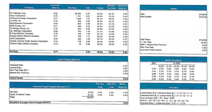
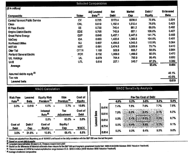
Let’s work through a couple of the calculations in the above screenshots. Take Central Vermont Holding on the top screenshot that has an observed Be of .74, the D/E is .444 and the t is .396. The little box on the bottom right hand side explains that Bu = Bl/(1+D/E) x (1-t). If there was no tax term, this the Bu would be Bu = Bl/(E/E+D/E) or Bu = Bl x Equity/Capital. This demonstrates that there is no Bd in the calculation shown in the top screenshot. With Bd included, the formula would be Bu = Bl x Equity/Capital + Bd x Debt/Capital. Therefore, the Bd is ignored. For the first screenshot, with taxes the calculation of Bu for Central Vermont is .74/(.444 x (1-.396) or .498. In the second table, the Bu is not defined in a footnote. However the formula appears to be the same. The Central Vermont Beta is .725 and the debt to equity is .728 in the second screenshot. Using a tax rate of 39.6% (not shown) produces Bu of .503. This again confirms that both of the tables ignore the Bd.
The average Bu in the first table is .49 and in the second table the Bu is .484. The market risk premium is 5% in the first table and 6.5% in the second table. The risk free rate is 3.6% in the first table and 3% in the second table. Therefore we can compute the Ku in both cases. In the first case the Ku is 3.6% + .49 x 5% or 6.05%. Ku is 6.15% in the second case. If there was no tax deduction on interest, this Ku would be same as the WACC no matter what how you re-lever the capital structure.
Beta on Debt Can be Derived from Bond Yields
The beta of debt (Bd) is often assumed to be zero in measuring the unlevered beta (Bu) as shown above. This means the Bd is also ignored in computing the all equity cost of capital (Ku). Without taxes, the formula for Bu is Bu = Be x Equity/Capital + Bd x Debt/Capital. If the Bd is assumed to be zero, the Bu and the Ku can be understated. I wonder if sometimes the debt beta is assumed to be zero because people don’t know how to compute it.
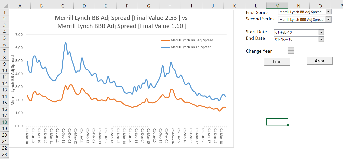
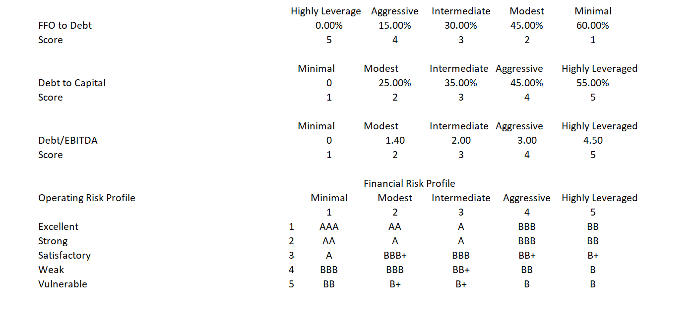
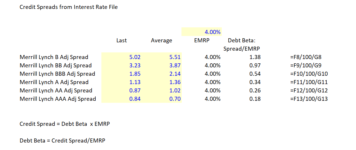
The debt beta can be derived from data on credit spreads given the EMRP and Rf. For example, the historic spread on BBB bonds is about 2% and the gearing of BBB companies is about 55%. The two screenshots below show the historic credit spreads and leverage of BBB companies. The first screenshot comes from the interest rate database. The second screenshot with the leverage and credit rating is from the credit analysis part of the website.
In the CAPM, the cost of equity is the risk free rate plus Be x EMRP. The cost of debt can be expressed in a similar manner with the formula Cd = Rf + EMRP x Bd, or if you are focusing only on the credit spread or risk premium, then CSd = EMRP x Bd. But for the cost of debt, we know everything except Bd. Restating the equation implies that CSd = EMRP x Bd or Bd = CSd/EMRP. If the credit spread is 2% and the EMRP is 4%, the the Bd is .5 (2%/4%).
The screenshot below illustrates how you can uses credit spread data along with an assumed Equity Market Risk Premium (EMRP) to derive the debt beta. The table includes different credit spreads from different bond ratings taken from the interest rate database file. The EMRP is the same estimated risk premium with all of the problems and issues that is used elsewhere in the CAPM. The table below illustrates how you can use the formula Bd = Credit Spread/EMRP to derive the debt beta for different credit spreads.
Implications of High Bd on Cost of Equity
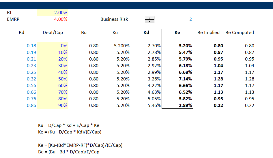
When the debt beta is high, the implied cost of equity and the Be can decline. This suggests that the cost of equity does not continue to increase with the debt to capital ratio. Instead, as the lenders take more risk, the risk of equity is reduced. Data on the relationship between debt to capital and credit ratings can be used to derive the beta on debt as a function of the market capital structure. By using the crude data on bond ratings for different debt to capital ratios along with the interpolate function, the Bd can be estimated for different capital structures. This is illustrated in the screenshot below. The table begins with the Bd and the debt to capital ratio. From two men that really did change finance, Modigliani and Miller, we can assume that Bu and Ku are independent of the capital structure. As Bu = Bd x Debt/Capital + Be x Equity/Capital, the Be = (Bu – Bd x Debt/Capital)/(Capital/Equity). Once Be is established, Ke = Rf + Be x EMRP and the cost of equity can be derived. Note in the table below that the Ke declines dramatically as the Bd and debt to capital reach high levels.
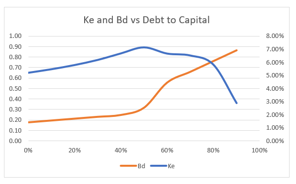
The graph below presents the Ke and the Bd as a function of the debt to capital ratio from the table above. For relatively low levels of Bd, the cost of equity increases with the debt to capital as is the traditional discussion in finance texts. But after the Bd increases to higher levels, the term Bd x Debt/Capital dominates the effect of Capital/Equity increasing in the formula Be = (Bu – Bd x Debt/Capital)/(Capital/Equity). This causes the Ke to decline as shown in the graph. The decline in cost of equity is consistent with the idea that equity is a call option and debt is a sold put option. With higher levels of debt the call option characteristics of equity with limited downside and large upside dominate.
Bu and Ku in Subsequent Webpages of this Section
Subsequent webpages develop various analyses of WACC and in particular the effects of the tax deductability of interest expense. In each of the cases, the analysis begins with Ku which in many cases is the WACC. To evaluate issues associated with WACC and the cost of capital along with the interest tax shield, it is assumed that both after tax free cash flow and Ku and Bu are constant. As the Enterprise Value of a company is the present value of future after tax cash flows (excluding the interest tax shield) and the Ku and Bu are independent of the tax shield, measurement of the cost of debt and the cost of equity in alternative scenarios. In various discussions involving the interest tax shield, I compare a no interest tax shield case with a case that includes an interest tax shield. You may say that if the tax rate changes, so should the after tax free cash flow that defines Enterprise Value. But throughout, I assume that the Enterprise Value is constant. You can imagine a case where a tax rate change does not affect operating cash flow because the firm is in a very competitive industry where consumers incur the costs and realise the benefits of tax rate changes. You can also imagine a case where the taxes on operating profits are different from the tax rate used in the tax shield.