This page demonstrates how you can compute sculpting from a curved DSCR in a project finance model that pays down the total amount of debt (determined from the debt to capital ratio) and at the same time meets an average debt life constraint and a minimum DSCR constraint. I used to think that sculpting meant the DSCR was constant where you could compute debt service as debt service = CFADS/DSCR and then subsequently compute the debt as the PV of the debt service. I was wrong because when the minimum DSCR and the debt is given you can model a series of changing DSCR’s. Then I thought that you could compute an DSCR from sculpting as with the LLCR formula, DSCR for Sculpting = PV of CFADS/Debt from Debt to capital. But I was wrong again. Hedieh told me that the correct sculpting method is to vary the DSCR until the DSCR is equal to the minimum DSCR as the minimum DSCR is below the LLCR. This means that the initial DSCR is above the LLCR and the DSCR gradually goes down until the DSCR falls below the LLCR and eventually down to the minimum DSCR.
The sculpting method discussed on this page computes factors that drive the an interpolated DSCR and uses a goal seek function with these factors to make sure the total debt is repaid. When using a goal seek to assure that curved DSCR re-pays the debt, alternative shapes can be developed with more or less extreme slopes in the DSCR. If the shape of the DSCR curve is too extreme, the average life will be very long. If the DSCR curve is less extreme and is flat, then the average life will be shorter and the equity IRR will not be as high as it could be. This page outlines how to apply a method to compute the optimal sculpting DSCR curve using a goal seek function to derive the curve and varying the shape of the curve with multiple scenarios. Note that if you want a higher Equity IRR, you want the dividends to occur at earlier periods.
Excel File that Demonstrates Curved Sculpting with Interpolate, Goal Seek and Data Table Method
Step by Step Approach for Computing Optimal Shape of DSCR Curve
The method for computing the optimal DSCR shape uses the interpolate user defined function, the goal seek function and a data table. In this section I describe the general process. I define terms including the LLCR factor; the final interpolation period; and, the curved DSCR.
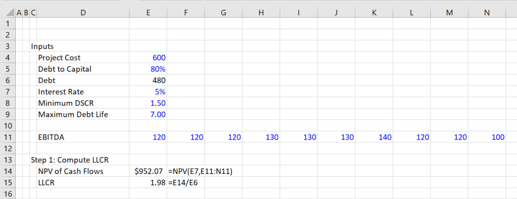
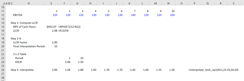
I have attempted to work through the above eleven steps and demonstrate that it is not really very difficult to implement this process. I use a very simple case with no taxes, and just a couple of simple cash flows. This example is shown in the screenshot below. Note that I have purposely changed the cash flow pattern over time.

The second step is to compute the LLCR from the PV of the Cash Flow. This is illustrated in the second screenshot below. There is a simple NPV calculation and then the LLCR is the PV of the cash flow divided by the amount of the debt computed from the debt to capital ratio.
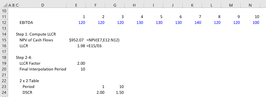
The third and fourth steps are shown in the third screenshot. This is where you create a 2 x 2 matrix and plug in a value for the LLCR and the end of interpolation period. The top row starts with 1 and ends with then end of the interpolate period. The second row ends with the minimum DSCR and starts with the LLCR x LLCR Factor.
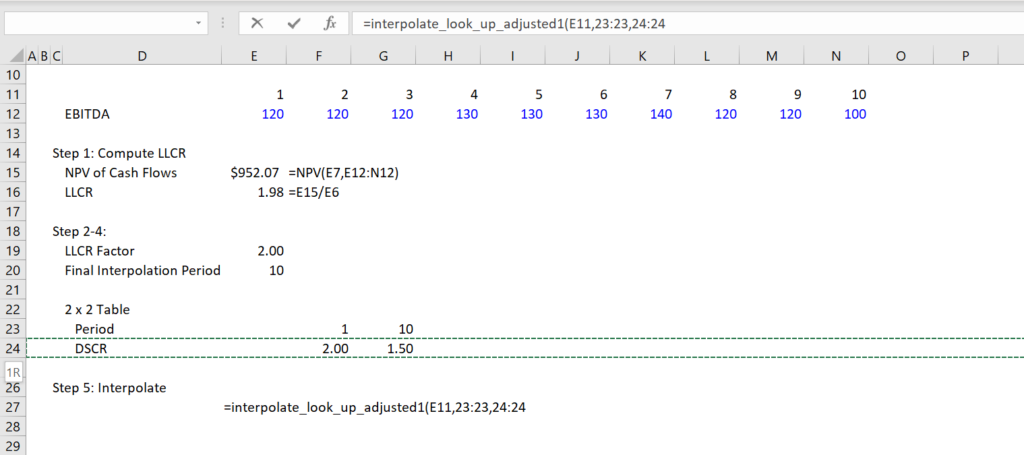
Compute Curved DSCR Using Interpolate
Step five is shown on the screenshot below. Here the curved DSCR is computed from the 2 x 2 table. You need to insert the lookup function into your file and use the 2 x 2 table.
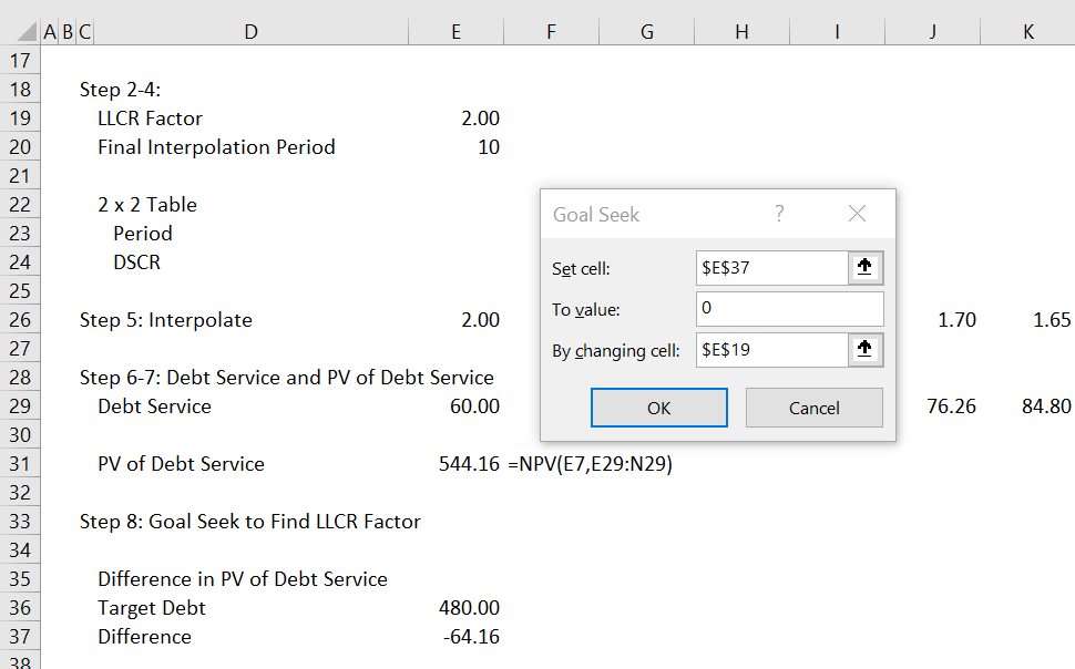
Step six and seven are illustrated in the next screenshot. You just divide the cash flow by the curved DSCR and then compute the PV of the debt service. Note that the PV of the debt service is not equal to the balance of the debt. This is where the goal seek comes into play.
Using Goal Seek to Find the Initial DSCR in the Interpolate
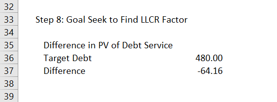
Step eight demonstrates derivation of the LLCR factor using the goal seek. You set the difference between the target debt and the PV of debt service to zero by changing the LLCR factor. When you create the goal seek, make a macro around the goal seek so that you can use it in the table.
Step nine demonstrates computation of the average loan life. For this computation you should create a debt account that begins with the target debt balance. The repayment is the debt service less the interest expense. The average life can be computed two ways as shown in the screenshot. One method is the sum of the balance. The second is to use the SUMPRODUCT of the debt number and the repayment divided by the debt balance.
