This webpage describes how to make a resource analysis of solar power, meaning an estimate of how much electric power can be produced in a given time period in a given location from solar panels which is a central part of solar investment analysis and solar financial models. The resource analysis I summarise below explains how to go to various websites and collect data on solar energy that hits a panel (in-plane energy, point of access energy). With this information on how much solar panel hits a panel along with estimates of how the particular panel affects the final performance in terms of ultimate electricity production — the performance ratio — you can compute net solar energy very easily.
To explain the resource analysis used in investment analysis, I try to explain factors that go into the measuring the performance ratio and the definition of the performance ratio is addressed. Terminology and calculation of things such as solar yield, performance ratios and temperature coefficients are also addressed.
In discussing the issues associated with solar, I will use the websites with solar data below. The website from the EU is really amazing. It uses data from PVGIS which is considered a good database if not the best. But using the link, you can not only find the basic data but also you can download hourly data that I use for storage analysis, for purchase evaluation and for other issues.
http://re.jrc.ec.europa.eu/pvg_tools/en/tools.html
http://pvwatts.nrel.gov/
https://globalsolaratlas.info/map
.
Power Point Slides for Solar
The power point file attached to the button below includes slides that work through some technical details of solar and integrating battery storage and then developing LCOE and Financial Analysis. If you are a banker or a developer or investor, I believe it is useful to get you hands dirty [se salir les mains] with some technical details such as the temperature coefficient, the wind shear facor, the shape of the power curve, the reason for DC versus AC capacity even if you would never dream of making any of this technical analysis. The technical details are explained in separate sections of the power point slides attached to the button below. The PPT slides begin with technical details and then move to LCOE and then move to financial models. This is done first for renewable energy solar and then for battery and storage analysis. I use this PPT file for the first section that works through LCOE and ultimately evaluates whether solar and batteries in some regions can compete on a stand-alone basis for data centres.
.
.
.
.
Excel Files to Work with Hourly Solar Data
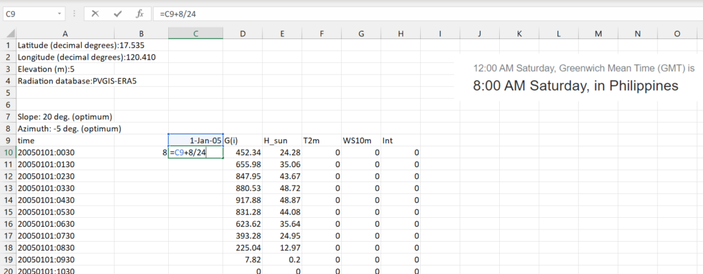
In addition to the above exercises, I have included a file in this section that demonstrates how to work with hourly solar data from PVGIS. In this file I use hourly data that you can download and demonstrate how the hourly data conforms to the summary data presented in the PVGIS website. In the file, you can see that the annual kWh per meter squared conforms to the sum of the hourly data over many years. In the file I also show how to work with dates so that you can quickly perform the analysis. The screenshot below the button for the example file shows that how to set dates after downloading the data. You should first establish the correct starting point that depends on GMT and then add 1/24 to the rest of the dates. As illustrated in the screenshot, this method of adding 1/24 to the date gets the data and the time.
.
Instructions for Downloading Files with Macros
.
Excel File that Demonstrates how to Analyse and Reconcile Hourly Data from the PVGIS Website
.
.
The next screen shot illustrates how to fill in the rows for dates and time in a few seconds. You can use the formula =if(prior=24,1,prior+1) for the hour in the day and also use the SHIFT, CNTL 2 to get the time.
.

.
.
.
.
.
Slides that Work Through Solar Power Issues and Why I believe that Solar Power Costs are a Revolution
In the file that you can download below I have put together my comprehensive thoughts on solar power and what I call the solar power revolution. I walk through the costs of Solar power and why solar power can be produced at nearly 1 US cent per kWh in some regions. The slides begin with the physcial characteristics of solar power and how panels are made. Then I move to the cost drivers and resource drivers. In this context I begin to explain how the compute the LCOE for solar using the PMT function. In computing levelised cost you can use the LCOE calculator attached to the button below if you do not want to go through all adjustments for inflation, taxes, degradation, different lives and other issues.
Power Point Slides Describing Resource Analysis and Financial Analysis of Solar Power Projects
.
.
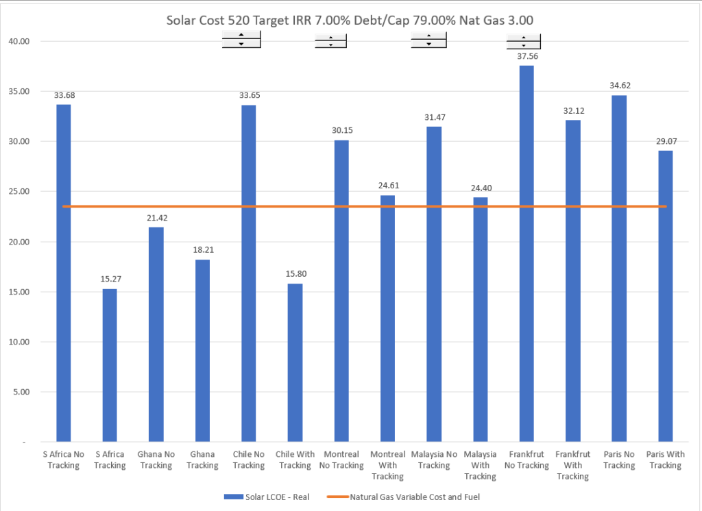
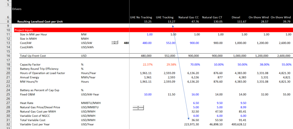
I have downloaded hourly data for South Africa, Ghana, Chile, Libya, Montreal, Paris, and Kula Lumpur using the EU website. I have done this so that you can understand the economics of solar and storage in different situations. For each of the locations I have downloaded the solar resource measured in kWh without tracking; the solar data with tracking and the net solar data after the performance ratio. The concepts and measurements are discussed much more below, but for now I have put files with this data so that you can evaluate costs, storage and other issues with the data. In the spreadsheet attached to the button below you can compare the levelised cost of solar in the different regions to the cost of natural gas. If you want a simple criteria, I think this is one thing you can do. Imagine that you put in panels somewhere and then you reduce the operation of natural gas. This is illustrated on the graph below. As shown on the graph, the LCOE depends on the cost of the solar project, the debt financing, the required equity IRR and other factors. The second screenshot illustrates a part of the LCOE calculation where the variable cost of natural gas is computed and compared to the real LCOE.
.
.
.
.
.
.
I have included a number of files on this page that demonstrate solar resource analysis issues. A few files are used in the resource analysis. The first file is write-up of the resource estimation process. that works through acquiring data, performance ratios and temperature coefficients. The second file is and excel file that extracts data on the cost of solar panels and contains a time series evaluation of solar costs. The third file is a set of power point slides that works through the solar resource estimates.
.
.
.
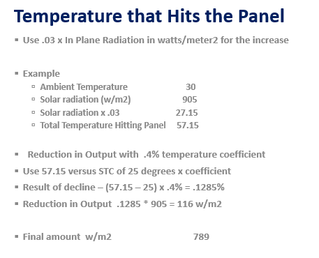
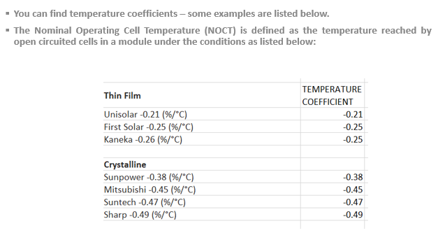
Temperature Coefficient
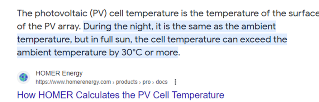
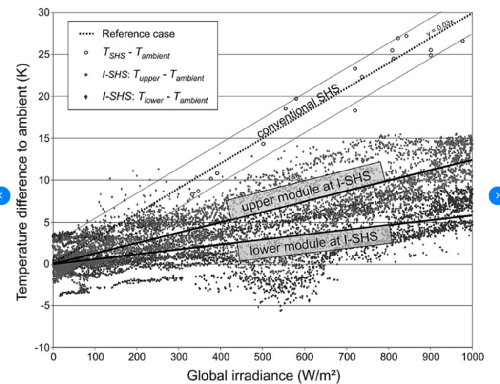
The discussion below demonstrates how to compute the temperature effect in the performance ratio from temperature coefficient. To do this you need to compute the temperature that hits the panel which can be called the PV Cell temperature. I have looked around for this as you can find the ambient temperature but not the increased temperature that drives the reduction in output. The relationship between the temprature increase and the solar output is demonstrated in the graph below.
.
.
.
.
Introduction — Resource Analysis in Renewable Energy and Output versus Availability Projects
.
In the example below the kWp is defined from the DC power at 1,000 W/M2 and it is also defined at 25 Degrees Celsius (Note the little footnote). The capacity is defined by this criteria and called STC, or Standard Testing Condition. The capacity is measured in DC, or direct current.
If the amount of sunlight was 1,000 W/M2 for every hour (including at night which is not so easy) and if the temperature that touches the panels was always 25 degrees, the theoretical capacity factor would be 100%. If the sunlight was 1,000 only for half the year, then the capacity factor would be 50%. This capacity factor is all before considering the performance ratio that I discuss below.
This multiplied by 8760 hours if you pretend the impossible situation, you would have a yield of 8760. The capacity factor would be 100%. The actual capacity factor is dramatically lower because:
- There is a lot less sunlight at night and when it is cloudy (see the graph below)
- The performance ratio is not 100% meaning that a Wp may only produce something like .85 W to the grid.


.

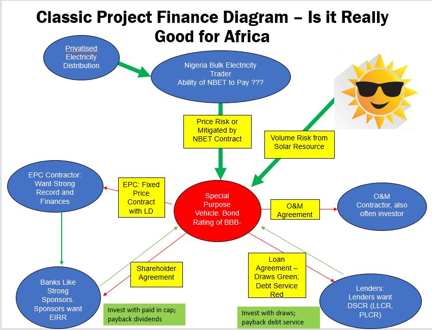
When purchased power agreements (PPA’s) are signed for plants that can be dispatched, the offtaker typically controls the dispatch. This means that imposing risks of dispatch on the investor would lead to wasted risk premiums where the investor would require higher prices that do not increase economic efficiency or reduce risk to consumers. Solar, wind and non-dispatchable energy in part depend on investment and operating decisions made by investors. For example, an investor could put a solar panel underneath trees in an area with cheap land and access to transmission. Another investor could use dual tracking and bi-facial panels to increase production. The effect of these investment decisions is generally attributed to investors through imposing volume risk to the investors as illustrated in the project finance diagram. Solar resource analysis is fundamental to the analysis of a solar project for many reasons.
This typical project finance diagram illustrates how solar power resource is not mitigated by other contracts (even though some people are trying make products that guarantee the production). I demonstrate this by the picture of the sun as the off-taker to volume risk which is not attributed to another party and is generally accepted by debt and equity investors. As this risk is not mitigated, it must be carefully studied and thing like P90 or P99 are part of the investment and modelling analysis.
Gross Solar Resource Estimates Using Public Websites
Solar power is different from other technologies in that you can perform a whole lot of resource analysis from the internet on specific projects in different locations. You can get estimates of solar resources; you can get historic data for computing P90, P99 etc.; you can solar capital get cost data; and you can find data for evaluation of the cost of capital. Some websites where you can find solar resource data include Retscreen, JRC, PVWATT and NREL (I think the top link is the best). To get the Retscreen data you need to download the retrscreen tool.
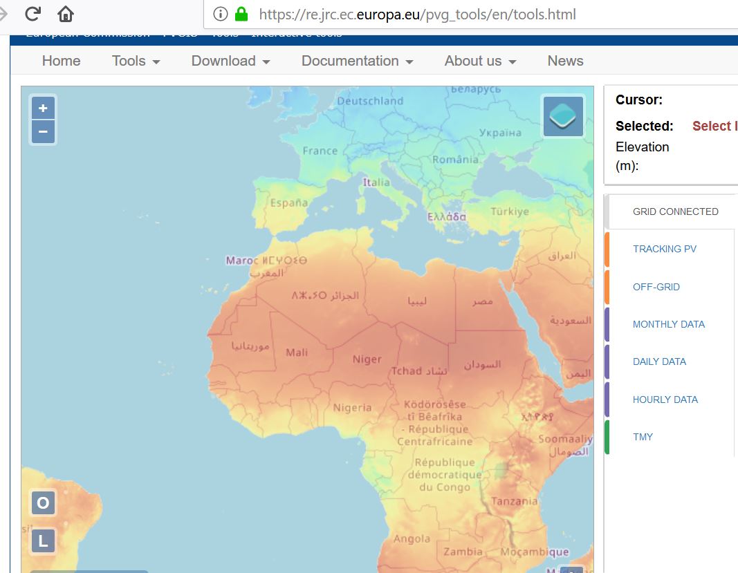
By far the best website is the one from the EU. You can even get hour by hour resource analysis for many years with alternative tracking. I begin the discussion by walking through the some solar analysis with this website to derive the solar power that hits the plane of a panel. This is called in plane irradiation and does not depend at all on the characteristics of the panel. After deriving the in plane irradiation I move to how the individual panel types can affect final performance through evaluating the performance ratio. I will walk through a few very simple ways in which you can assess the resource analysis without being a fancy engineer. I compare the energy yield that comes from a project in Norther Nigeria with a project in Scotland. The files and videos below walk through analysis of the solar resource, meaning the amount of solar energy that is available at different places in the globe. An file the works through computing solar production from various sources can be downloaded by pressing the button below.
When opening this website, you get a nice map and then you can press on the area to find the resource like your are searching on a google map. The map has different colours that demonstrate the amount of solar power in different areas with the blue areas having the least and the brown areas having the most.
.
.
In solar resource analysis, all costs including If there were no clouds or dust and the sun did not have sun spots, then the amount of solar power (extra terrestrial that sounds like science fiction) could be computed direct from longitude and latitude. But clouds and other things complicate the calculation. These conditions can be measured with satellites that are going around the globe and measuring all sorts of atmospheric conditions. Because of all of this, you can click on a google map type picture and then get the amount of solar power per kW per meter squared in different places. financing costs and operation costs are fixed (unless you can imagine a cost that changes when the sun shines more or less). If you have twice as much solar output the cost is halved. To demonstrate how the resource affects the economics of solar power, imagine two factories with the same fixed cost and no variable cost. One factory produces half as much as the other. The factory with lower production must receive twice the price.
To illustrate solar resource estimation, lets do a very simple comparison between Scotland and Northern Nigeria. After clicking on the location when you use the EU website, you can look at the grid mounted or the axis tracking options. After you press the option to visualise results, you see a few statistics on the left hand side. To introduce resource allocation, concentrate on the in-plane radiation that hits the panels. The in-plane irradiation that hits the panel is expressed in kWh/m2. As solar panels are defined to be at 100% of there capacity when the irradiation is 1000 watts/m2 and when the temperature is 25 degrees as explained below. If each hour of the year produced 1000 watts/m2, then the amount of power over the year would be 8760 hours multiplied by 1000 watts or 8,760,000 watt hours. Dividing by 1,000 produces 8760 kWh/m2.
This means that in-plane yield in kWh/m2 divided by 8760 gives you the capacity factor: 2780/8760 is 31.7%. You won’t find much better places than this. Note that this includes single axis tracking. Now, with tracking, the yield per kWh on the plane of the solar panel is only 1,010 kWh/m2. This produces a capacity factor of 11.52% (1010/8760).
.
The capacity of a panel is defined by something called kWp or MWp where the p represents peak and the measured instantaneous DC capacity is measured at a term called Standard Testing Conditions or STC. Standard testing conditions are how much power would be produced by a panel if there was solar energy touching the panel of 1,000 W/meter squared (measured with a flash test) and the temperature is 25 degrees Celsius.
If the average amount of energy over the year is 150 W/meter squared and the temperature is always 25 degrees and there are no losses from wiring, snow, shading, dust etc., then the capacity factor would be 15%. This is simply the average irriadiation of 150 divided by the maximum irriadiation of 1000. It is 150/1000, where the 150 is the average production per hour over the entire year and the maximum production is the 1,000 Watt defined as part of the STC.
In solar resource analysis, the capacity factor and the yield measure the same thing. In my example with an average production of 150 W/meter squared, you can calculate the yield. The yield is often uses in the industry and has the same information as the capacity factor. In this case, the yield would be 150 x 8760/1,000 or 1,314 kWh/kW. The units for yield are really hours and the yield divided by the hours in a year — 8760 — is the capacity factor. These simple equations are summarised below:
Capacity Factor = Average Production (kWh per year/8760)/Capacity (kWp)
Yield = Total Production per Year/Capacity (kWp)
Performance Ratio
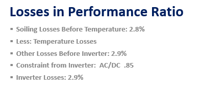
The performance ratio should measure solar production effects of anything other than irradiation that hits the plane of the panel. Once the plane is hit by the sunlight, all of the things that can go well or badly in producing the final production are part of the performance ratio. I compute the ratio a little different than others using the formula:
Performance Ratio = final capacity factor/in-plane capacityr factor
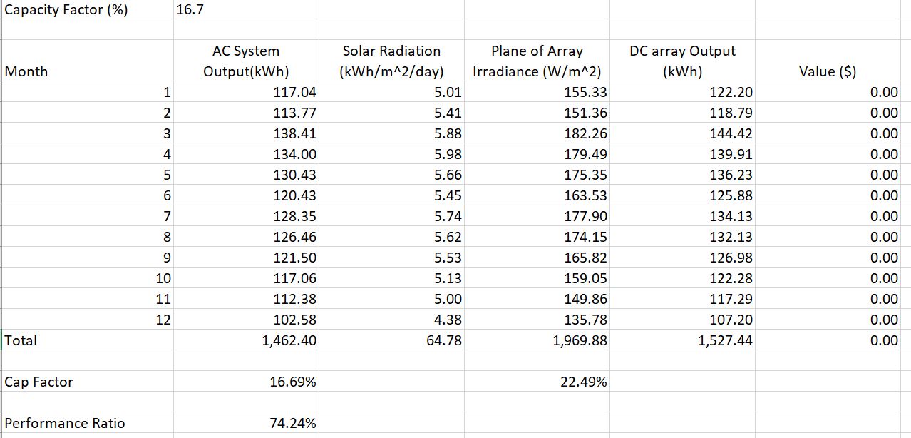
The capacity factor calculation for in-pane irradiation is illustrated in the screen shot below. In this case the capacity is 1,000 Wp. In the AC System column at the left, the total generation of 1462 kWh can be divided by 8760 to come up with average production of 166.89 Wh. The 166.89 divided by the capacity of 1000 Wp gives the capacity factor of 16.9%. This is the numerator of the PR calculation. The capacity factor at the plane of the solar panel can also be computed as discussed above. This is the total w/m2 over the year of 1969.88 x 1000/8760 to arrive at the average irradiation. This number is again divided by 1000 giving 22.49%. The performance ratio is 16.69%/22.49% giving 74.24%
.
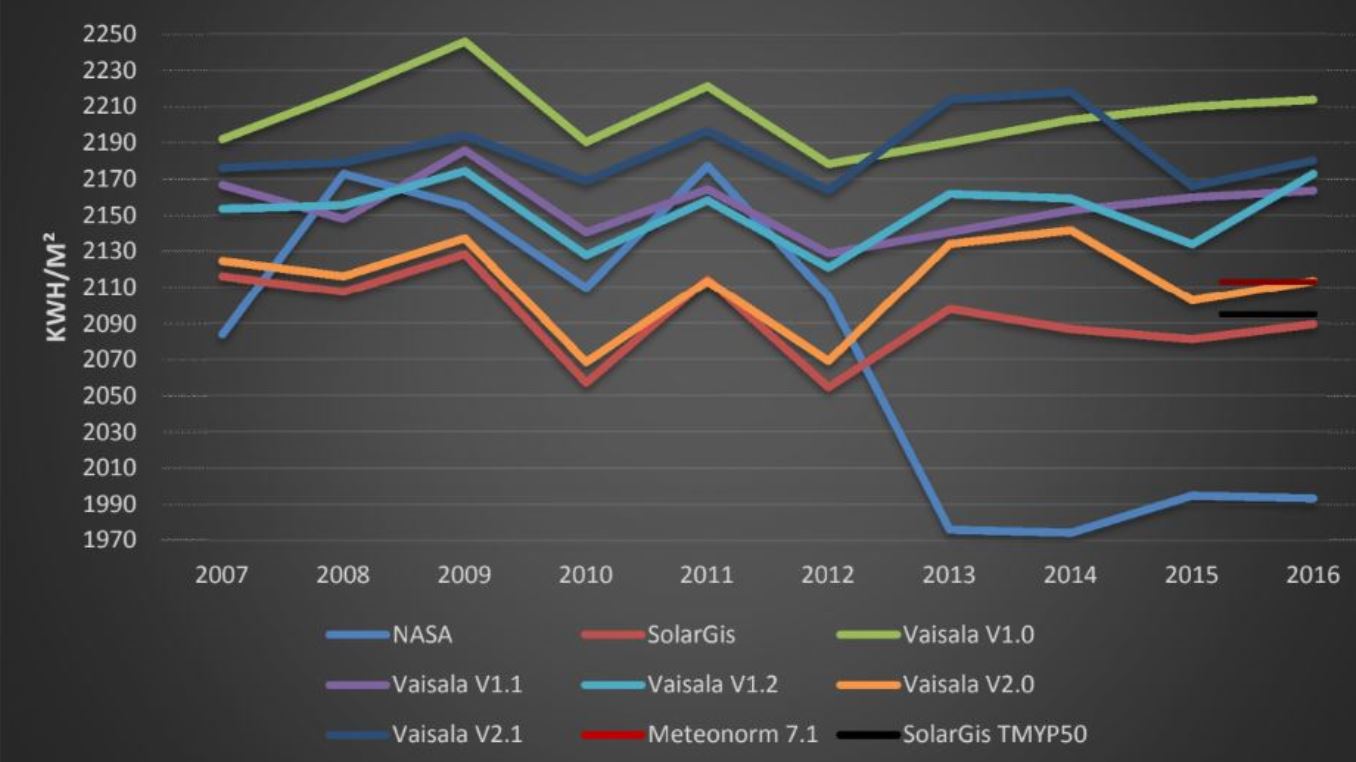
It should be clear that the actual production of solar power depends on the performance ratio as well as the amount of sunlight. The performance ratio reflects characteristics of the solar panel and other equipment including the reaction to temperature, losses and other factors. The screenshot below (taken from the above file) illustrates that different sources of solar data and different estimates of the performance ratio can result in large differences in estimated solar production. The performance ratio is the final capacity factor divided by the point of access capacity factor that comes from the solar analysis and is independent of the solar panel type. I have included a couple of actual examples of the performance ratio from financial models in the screenshots below.

.

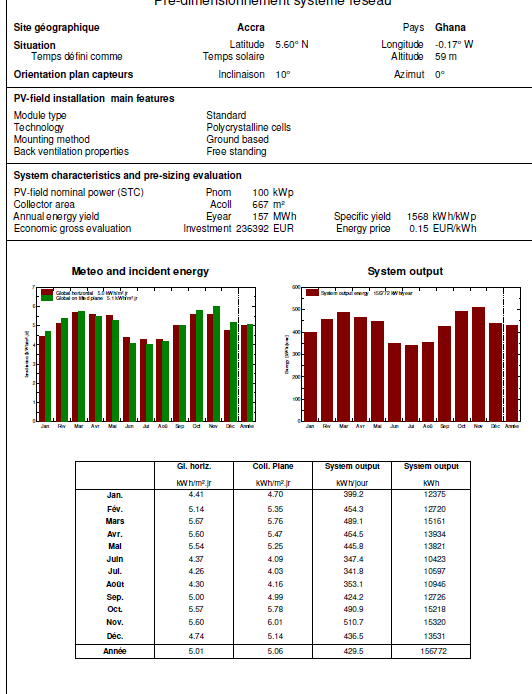
For an exercise, you can compute the PR for the PVSYST case below.
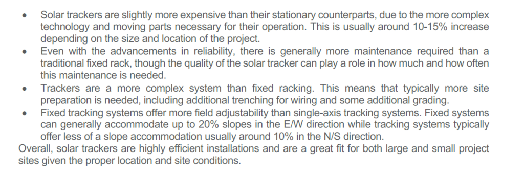
Tracking
.
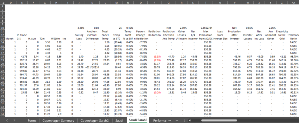
Computing Solar Output from Hourly Data with Temperature Coefficient
Two buttons below are attached to exercises that work through a system analysis with loads and solar power. You use the temperature from the PVGIS and an assumed temperature coefficient to derive the effect of temperature on energy production. You also add in the losses so you can evaluate the total production.
.
.
.
.
.
Interpreting Solar Irradiation From PVSYST and Other Sources
The discussion below shows how to take various sources of solar power and then adjusts them by the performance ratio (temperature, losses etc.). With the performance ratio you can compute the solar yield in a crude but reasonable manner.
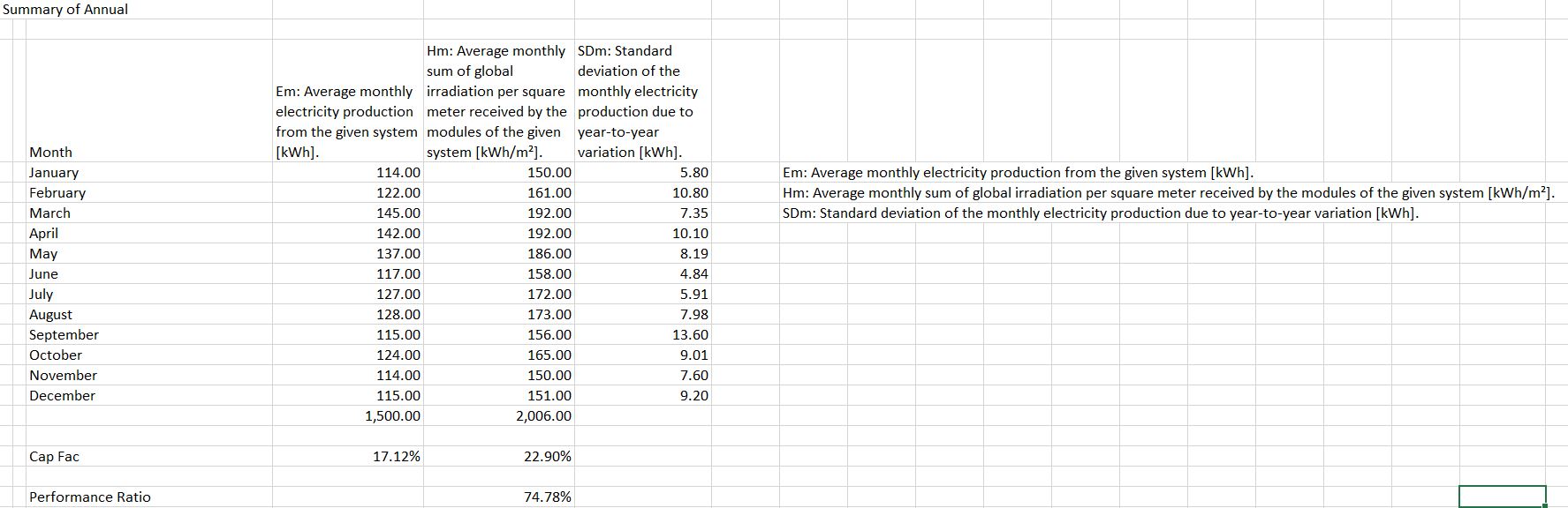
In this section I explain how you can compute the performance ratio using different sources. The first example is the EU website which reports Em as the final production that is sent to the grid. Hm is the solar production received by the module. The screenshot demonstrates how the performance ratio is the final production capacity factor divided by the energy that hits the modules (panels). This is again taken from the solar yield file that is available by clicking on the button in the last section.
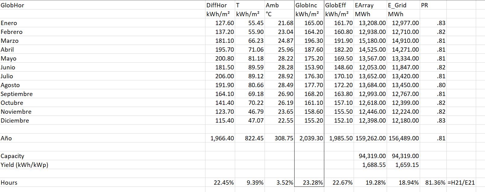
The second screenshot shows outputs produced by the PVSYST model. There are some names that are tricky to interpret. The units are different for the GlobInc column and the E_Grid column. But don’t worry. Just compute the capacity factor and understand which column reflects the amount of solar production that hits the panel. In the example below the performance ratio is 18.94% divided by 23.28% or 81.36%.
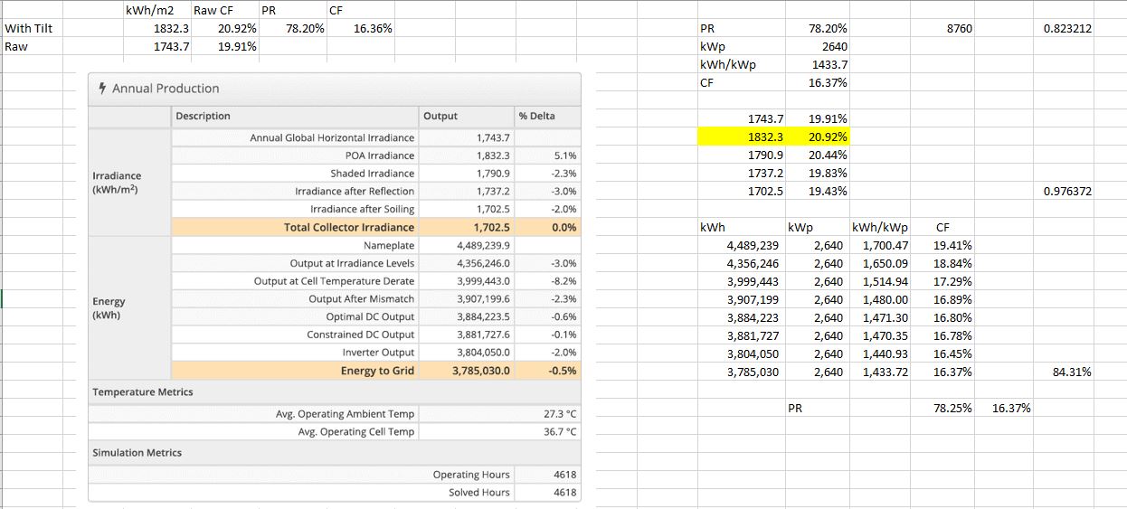
The third screenshot shows the output from Heilioscope. As with the PVSYST you should find the radiation that hits the collector and also the energy to the grid. You should get them in the same units by computing the capacity factor. Then you can divide the final energy to the grid by the collector capacity factor (by understanding STC and 1,000 W/m2).
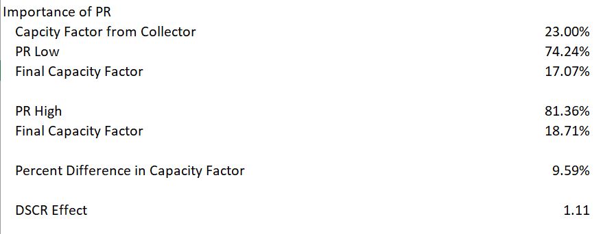
The second screenshot demonstrates the importance of the performance ratio and shows the DSCR required to cover uncertainty in the performance estimate. The DSCR is computed as 1/(1 – Percent Difference).
Working with Hourly Solar Data
If you are working with mini-grids or home solar power systems or other battery storage applications, you should be more interested in hour by hour production that can vary from hour to hour and day to day.
Videos Describing How to Evaluate Solar Production
I have made a couple of videos below that describe how to use websites in developing resource estimates of solar power. The videos include explanation of how to download data from PDF files and evaluate the implied performance ratio and the capacity factor in different places.
[wonderplugin_video iframe=”https://www.youtube.com/watch?v=mIS5hkXx5I0″ videowidth=600 videoheight=400 keepaspectratio=1 videocss=”position:relative;display:block;background-color:#000;overflow:hidden;max-width:100%;margin:0 auto;” playbutton=”http://edbodmer.com/wp-content/plugins/wonderplugin-video-embed/engine/playvideo-64-64-0.png”]
[wonderplugin_video iframe=”https://www.youtube.com/watch?v=IExGu1mk5c0″ videowidth=600 videoheight=400 keepaspectratio=1 videocss=”position:relative;display:block;background-color:#000;overflow:hidden;max-width:100%;margin:0 auto;” playbutton=”http://edbodmer.com/wp-content/plugins/wonderplugin-video-embed/engine/playvideo-64-64-0.png”]
- Solar Yield Analysis.xlsm
- Performance Ratio Analysis.xlsx
- Hourly Data from Weather Stations:
There are a lot of solar pages related to the files and the methods described below.
- The featured solar model page that is linked to this sentence includes completed finance models.
- There is also a file that allows you to automatically download panel prices and the price of silicon used in manufacturing the panels which is linked to this sentence.
- There is a webpage that works through resource issues including the performance ratio and how to find the best data on solar energy that hits a panel.
- There is a webpage that describes computation of the P50 versus P90, P99 etc. with some examples.
- There is a webpage that describes the arcane tax equity aspects of financing tax equity in the U.S.
- There is a page that works through how to consolidate multiple roof-top installations into a aggregate file.
Files associated with Lesson Set 1: Solar Resource Analysis
The first step in the lesson set is evaluating solar resource. The files first set of files involve putting solar data together in a file. The basis for computing P99 etc is the NREL website and download the zipped file for a location (sorry that this is only U.S. data). The first set are files work with detailed raw data from NREL that has hourly data from 1991-2010. If you try this, go to a file and then run the MOVE macro and put each of the in a file. You can do this by opening the template file below and pressing SHIFT, CNTL, X. In addition to files that work through the solar data I have included a database of actual solar projects that is called the solar database. This database allows you to evaluate P90, P99 etc. on the basis of actual data.
[wonderplugin_video iframe=”https://www.youtube.com/watch?v=UUP1v2Od59E” videowidth=600 videoheight=400 keepaspectratio=1 videocss=”position:relative;display:block;background-color:#000;overflow:hidden;max-width:100%;margin:0 auto;” playbutton=”http://edbodmer.com/wp-content/plugins/wonderplugin-video-embed/engine/playvideo-64-64-0.png”]
Get Detailed Solar Data.xlsm
There are a lot of solar pages related to the files and the methods described below.
- The featured solar model page that is linked to this sentence includes completed finance models.
- There is also a file that allows you to automatically download panel prices and the price of silicon used in manufacturing the panels which is linked to this sentence.
- There is a webpage that works through resource issues including the performance ratio and how to find the best data on solar energy that hits a panel.
- There is a webpage that describes computation of the P50 versus P90, P99 etc. with some examples.
- There is a webpage that describes the arcane tax equity aspects of financing tax equity in the U.S.
- There is a page that works through how to consolidate multiple roof-top installations into a aggregate file.
Solar Project Finance Model
The second lesson set involves a step-by-step project finance analysis of a solar project. Building a solar project finance model is not very different than some of the other lesson sets that are described in the page name “Project Finance Exercises”. The lesson set therefore focuses on incorporating solar resource analysis into a project finance model.
These Files are Available on the Library. Get them by e-mailing edwardbodmer@gmail.com
- Solar Sensitivity Analysis.xlsm
- Assumptions.xlsx
- Solar Pre-tax Cash Flow.xlsm
- Solar Project Finance Model – Cash Flow Equations.xlsm
- Solar Project Finance Model – Basic Financing Equations.xlsm
- Solar Plant Characteristics.xlsm
- Solar Project Finance Set-up.xlsm
- Solar Project with Financing Inputs.xlsm
- Solar Project Finance Model – Basic Financing Equations.xlsm
- Solar Project Finance Model – Cash Flow Equations.xlsm
Levelised Cost of Electricity and Currency Analysis in Solar Project Finance
- Currencies in Solar Model.xlsm
- Solar LCOE Model.xlsm
- 23. Carrying Charge Analysis Revised.xlsm
- Solar Annual Model.xlsm
- Solar Sensitivity Analysis.xlsm
- Solar Model Version 3.xlsm
In the discussion below I try to walk you through how to find the data and then compute the levelised cost of electricity from solar power in different places. While the levelised cot of electricity can be a controversial statistic, I argue that if the total cost of producing power from solar energy covering all of the fixed costs is less than the marginal cost of electricity, then solar is clearly economic. To be more precise, if the real LCOE (that is, in today’s currency) for solar is less than the variable cost of producing power from other sources, then it is better to throw in a bunch of panels and reduce energy cost.
If you go to the page that describes LCOE, you can see the relatively simple formulas that can be used to compute LCOE. The formulas require capital cost, capacity factor, O&M cost and the carrying charge rate. This page explains two of the key factors in solar analysis — the capital cost of solar and the capacity factor. The process of computing the solar LCOE is described in detail in the attached using the First Solar Case Study (It is a bit long so I am told nobody will read it).
.

Videos associated with Lesson Set 1: Resource Analysis and Financing of Solar
| Subject | Excel File | Video Link | Chapter Reference | Page Reference | ||||||
| Finding Solar Irriatiation Data | Solar Resource Analysis | |||||||||
| Working with Hourly Data | NREL Template | https://www.youtube.com/watch?v=bqQdQhVl_eY | ||||||||
| Computing P90, P75, P50 etc. from Irradiation | P90, P95, etc. | |||||||||
| Computing Capacity Factors from Irradiation | Net Yield Analysis | https://www.youtube.com/watch?v=PguZQz-RtDw | ||||||||
| Incorporating Performance Ratio Uncertaintity | P90, P95, etc. Multiple Factors | |||||||||
| Timing in Solar Project Finance Model | Timing in Solar Model | https://www.youtube.com/watch?v=eQYUuKQ0k94 | ||||||||
| Yield, Degradation and Capacity in Solar Model | Yield and Capacity in Solar Model | |||||||||
| Operating Analysis in Solar Model | Operations Analysis | https://www.youtube.com/watch?v=PGgfKaSJHBA | ||||||||
| Working Capital In Solar Model | Solar Working Capital | https://www.youtube.com/watch?v=r85rhfB9NRQ | ||||||||
| Financial Related Inputs and Financial Model Structure | Solar Financing Inputs | https://www.youtube.com/watch?v=–iThEBTMSo | ||||||||
| Financing Equations | Solar Financing Equations | https://www.youtube.com/watch?v=DfOUjWw-p6c | ||||||||
| Cash Flow Equations | Solar Cash Flow Equations | https://www.youtube.com/watch?v=vkLfOW_vwH0 | ||||||||
| Presentation of Annual Data and Debt Cash Flow | ||||||||||
| DSRA in Solar Model | ||||||||||
| Preparing Balance Sheet and Audit Checks | ||||||||||
| Resolving Circular References in Solar Model | ||||||||||
| Creating Tornado Diagrams in Solar Model | ||||||||||
| Adding Inflation to a Project Finance Model | ||||||||||
| Including Depreciation on New Expenditures | ||||||||||
| Using Models to Create Templates | ||||||||||
| Working Capital in Project Finance | ||||||||||
| Scenario Analysis | ||||||||||
| Tornado Analysis | ||||||||||
| Tax Equity and Flip Structures | Tax Structuring Model | |||||||||
| … | …………………………………………………………………………… | … | …………………………………………………………… | … | ………………………………………………………………………………………. | … | ……………………………………. | … | ………………………………… |