This page explains how to use a Normal Distribution, a Weibull Distribution, a log-Normal distribution, or a simple flat distribution in Monte Carlo Simulation. With the RAND function in excel or the RND function in VBA, you can apply alternative distributions to the Monte Carlo simulation. Alternative distributions allow you to assess risk in different ways and do things like including skewed distributions and fat-tailed distributions. My general point about Monte Carlo simulation and indeed many other subjects is that you should not be afraid and you should mess around with excel sheets. The reason for use of the normal distribution is that the volatility comes from standard deviation and can be used to create probability distributions. When other distributions are used, the volatility does not have the same meaning.
Three alternative distributions illustrated below include a (1) a simple distribution with constant probabilities across the range; (2) the normal distribution; (3) a log-normal distribution and, (4) alternative distributions that can be created from the Weiblull distribution.
Normal Distribution
In the case of a constant distribution, you can simply use the formula (RAND()-.5) instead of the NORMSINV() in the time series equation. In this case, when you multiply the (RAND()-.5) by the volatility, you can use the volatility to estimate the probability of being above or below a level.
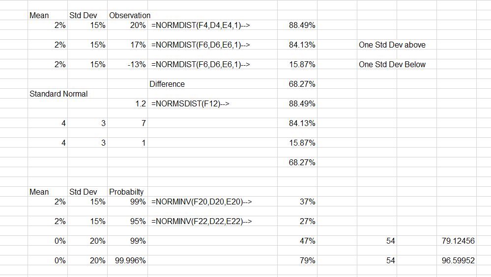
A couple of files with some general exercise on working with the normal distribution are available for download below. The screen shot below shows various ways the normal distribution can be used. The numbers in the box show that when you either add one standard deviation to the mean AND deduct one standard deviation from the mean, you achieve the famous 68% probability number.
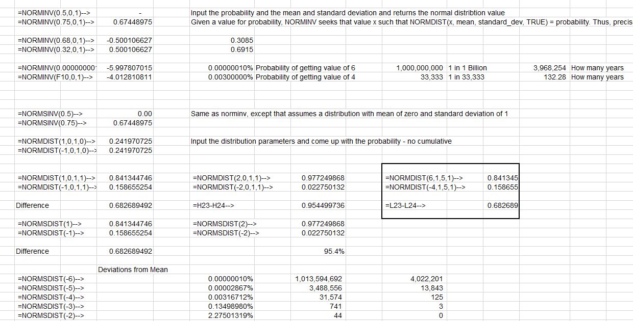
The second screenshot below shows how the NORMDIST and the NORMINV functions work. Note again that you can enter the standard deviation and achieve the 84% or 16%. You can do the inverse where you put in the probability and arrive at the value of the normal distribution.
If you want to download files that include exercises to work with the normal distribution you can press the couple of buttons below.
Exercises in Working with the Normal Distribution and Demonstration of Mean +- Standard Deviation is 68% Excel File with the Log Normal Distribution where Rate of Return Rather Absolute Levels are Used
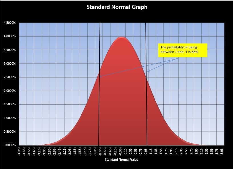
Creating a standard graph of a normal distribution with bands for the standard deviation is included in the second graph.
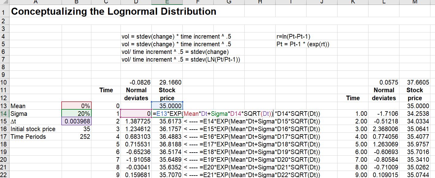
Log-Normal Distribution
The method of using the log-normal distribution rather than simple distributions is shown below. The log-normal distribution will not become negative and is demonstrated in the formula in the screenshot below.
If you use a log-normal distribution then you can first compute the rate of return. After that, compute the standard deviation of the rate of return that you can use for volatility. In the Monte Carlo simulation, you can use the formula:
Value (t) = Value (t-1) * EXP(Volatility * NORMSINV(RAND())
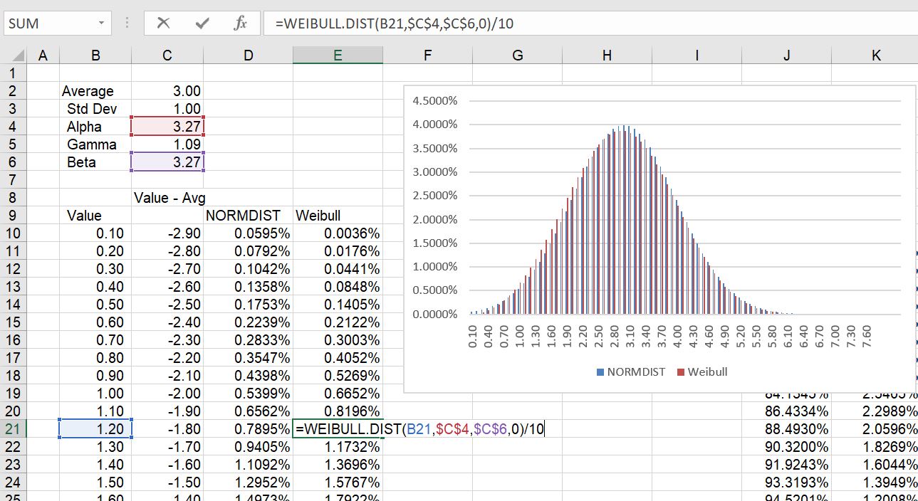
Weibull Distribution
In this section I show how to use the Weibull distribution in the context of Monte Carlo simulation. The Weibull distribution is driven by an alpha and a beta parameter in excel and I am not going to put the equation below. You can think of this as analogous to the normal distribution which is driven only by the average and the standard deviation. The file with the Weibull distribution is available for download by pressing the button below.
The Weibull distribution is sometimes used in wind analysis to project the capacity factor of wind over the course of a year given the average level of the wind. This is because wind movements from hour to hour an not normally distributed. To see why wind is not normally distributed, just think of how many times somebody has told you that the wind speed is negative today (it may change directions, but it is not ever stated as a negative number). On the other hand, when it is really windy, the wind speed is very high. If wind had a normal distribution, there would be negative wind speeds to offset the very high wind speeds at other times as the distribution is symmetric.
When working with wind speeds the Weibull distribution is often used. This is a more flexible distribution where you can make things skewed; you can make things have a fat tail; and you can make a symmetric distribution that looks like the normal distribution. In wind, the following parameters are typically used (I don’t know why, but people must have done a lot of curve fitting for this):
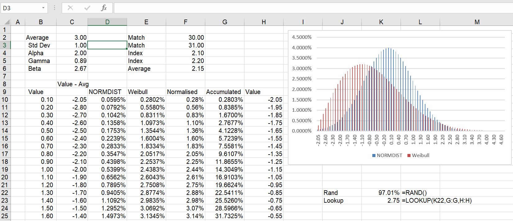
Alpha = 2.0
Gamma = .89
Beta = Gamma x Average Wind Speed
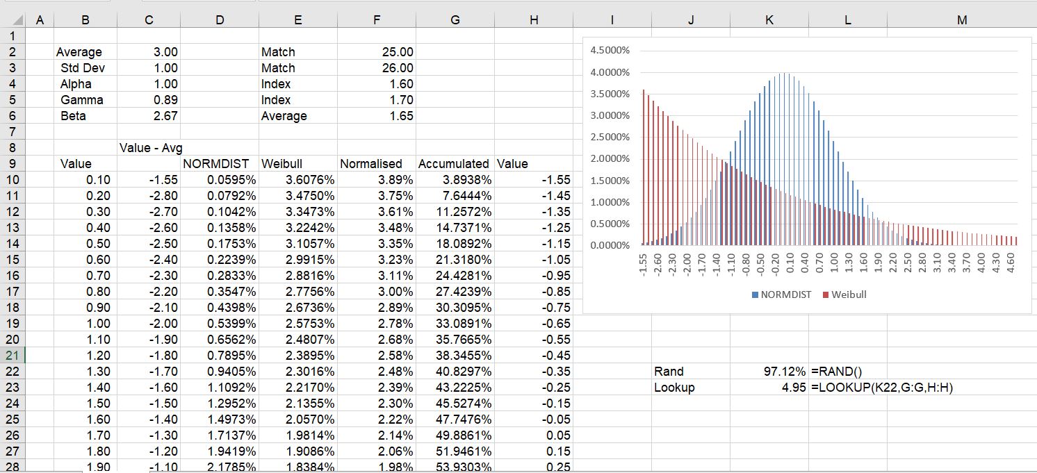
To illustrate how the process works, I compare the Weibull distribution using different parameters with the normal distribution. In the first case, the normal distribution is compared to the the Weibull distribution with an Alpha and Beta that result in a similar distribution. Using this situation, you can create something similar to the NORMINV function by changing the x-scale and normalizing the scale. This demonstrates that in the case of the Weibull, the values cannot be negative.
When the wind parameters with and alpha of 2.0 and a gamma of .89 is used, the distribution changes as shown below. In the diagram below, an adjusted standard value is shown has a mean of zero. This can be used with the LOOKUP function to derive something like the NORMSINV function. That is to say, you can put the LOOKUP function into the time series equation instead of the NORMSINV with the table of Weibull values.
The final chart shows the Weibull distribution with different parameters that produces something like a level distribution. This illustrates the flexibility of the distribution to model alternative situations.