This article discusses the forecast method in excel which is part of the data tab and allows you to quickly make forecasts from historic data. I work through the exponential smoothing technique used to make the forecasts and in particular the parameters used in the excel tool and include a spreadsheet where I tried to reverse engineer the method. Using forecasts from the parameters implied by the excel forecast I try to back out the implied parameters.
One of my students asked me how the excel forecast works. At the time I had no idea that there was even a forecast in excel. Then I saw the excel forecast which looks pretty cool. When you go to the internet and google forecasting in excel, you get a whole bunch of discussion of how you can press a couple of buttons and get some forecasts. A lot of the explanations also tell you how you can use the FORECAST.ETS function and retrieve statistics such as alpha and beta and the root mean squared statistic. These explanations also tell you how you can get confidence intervals from the FORECAST.ETS.CONFINT function. One website called real statistics does walk you through how to make your own forecast (and I used this). I originally worked on this whole forecasting business because of a question from a person in one of my classes who wanted to know how the confidence intervals are calculated.
But here is the problem, the ETS.FORECAST is a black box. None of the websites tells you in detail how to replicate the forecast and the confidence intervals in detail. This is a big problem because the forecast is made from exponential smoothing which is a very simple process. When I have tried to make my own model in the worksheet file below I have not been able to replicate the forecast parameters in excel.
Maybe this is because I am just stupid (probably). The forecasts for different GDP per capita growth look good, but I think there is something very odd with the excel reported parameters from the forecasts. First, the forecasts often have a clear trend. But the trend parameter — the beta — reported in the ETS.FORECAST.STATISTICS is .001. I really may be missing something here so I must be careful about my statements. Maybe they are mis-modelling the beta parameter, but I don’t think so. The really bad thing about this is that the beta parameter is by far the most important factor in making a forecast. Without the beta parameter the exponential smoothing forecast is a flat line.
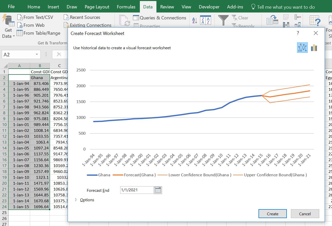
The file that you can download by clicking the above button begins by demonstrating how the excel forecast tool works like all of the other websites (this is really no big deal). In seconds, you can make a time series forecast now in excel. You just select a series of data adjacent to a series of dates, and you get a series of forecasts along with a confidence interval. You can export the forecast to a separate sheet. The only question is what are the techniques that excel uses to do this. First, just get some data. You can get the file for the economic variables and make forecasts for things like GDP per capita, population, life expectancy etc. The only thing you do is to select the date and then go to the DATA ribbon and then click on the forecast tab as shown below. This uses the FORECAST.ETS function.
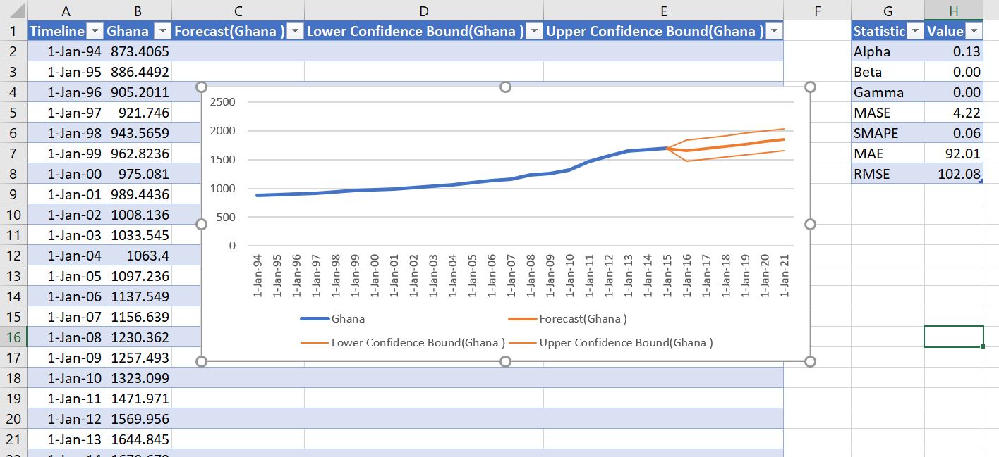
Once you do this you can select the option to list the statistics. This is computed with the FORECAST.ETS.SEASONALITY function. An example of this output is shown below.
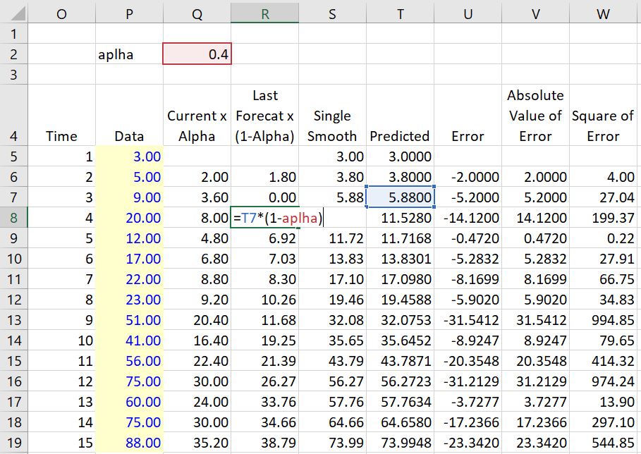
This is all quite boring. The real question is how are the forecasts made. To illustrate how the forecast is made using exponential smoothing, begin with a simple case without a trend. This forecast will be the same for each year of the forecast. The forecast is a weighted average of the current data value and the prior forecast. The current data is given a weight of alpha and the prior forecast is given a weight of (1-alpha). This means the alpha is multiplied by the current value and the prior forecast is multiplied by 1-alpha as illustrated below. The illustration demonstrates that the forecast remains constant. The absolute error and the mean square error can be used to find the best value of alpha with a data table or with a macro. The column Q has the alpha multiplied by the current data value. The error is the difference between the predicted value and the actual data.
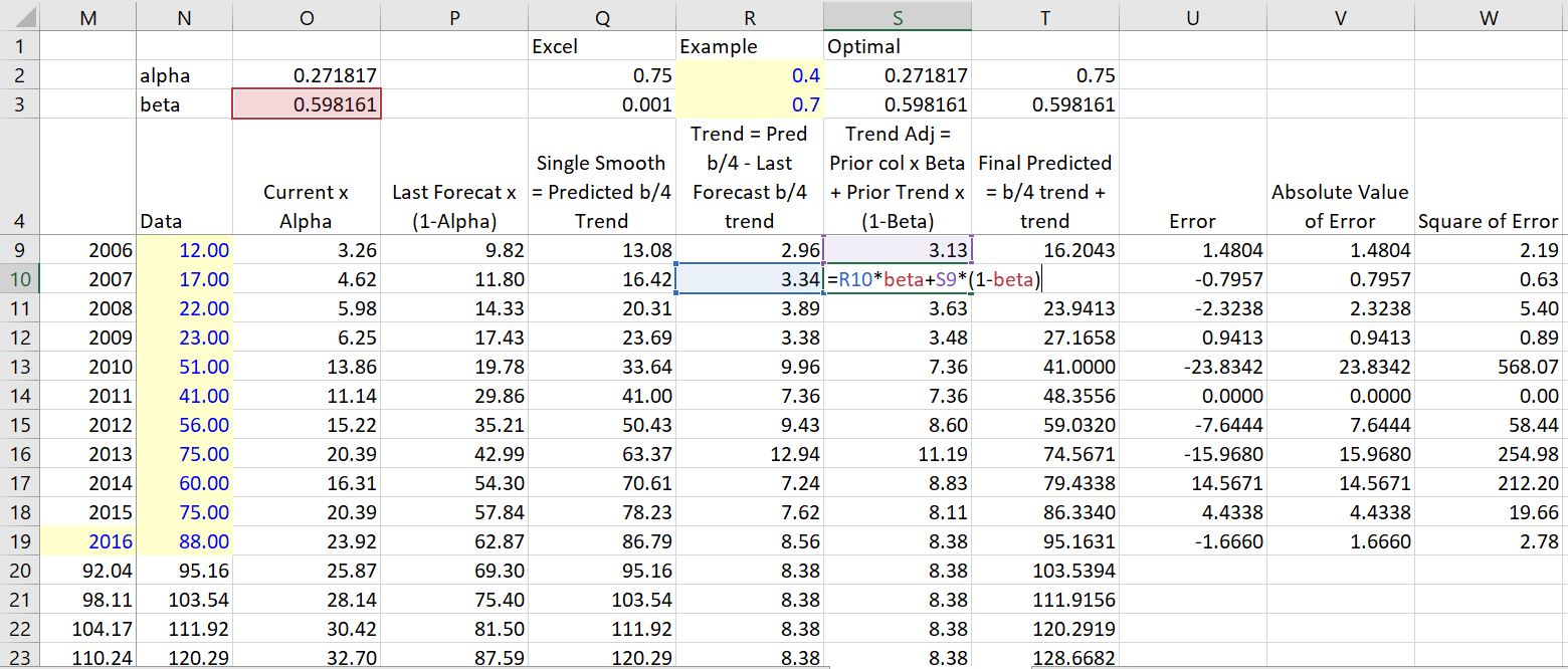
It is more interesting to include a trend in the analysis then to only weight the prior forecast and the current value. To do this trend analysis you can include a beta factor. This beta or trend factor is applied to the trend rather than the forecast. The trend is computed as the difference between the prior value without a trend and the current value without a trend. These are computed in a similar as the simple exponential smoothing. For me, the key is to have the correct number of columns. One column is for the exponential smooth without the trend. The next computes the trend. Then, finally the trend forecast can be computed.
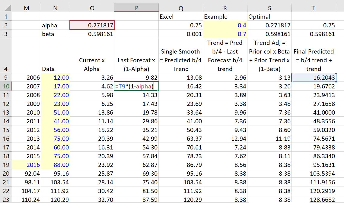
The single smooth is the last forecast value without the trend plus the current value multiplied by the alpha as shown below.

It is more interesting to understand the trend in the analysis. To do this you can include a beta factor. This factor is applied to the trend rather than the forecast. The trend is computed as the difference between the prior value without a trend and the current value without a trend. These are computed in a similar as the simple exponential smoothing.
I demonstrate how the forecast is made for GDP per capita in many different countries in the video below. By pressing the spinner button you can see the forecast results and how the trends occur and how the variance of the forecast is affected by the variability in the historic prices and the size of the alpha and beta parameter. This is in the forescast page of the file below. In the next sheet of the file I show I have replicated the excel forecast and the alpha and beta parameters are completely different. I use either a goal seek or a solver technique to match the forecast. This replication results in very different parameters from excel and shows how the excel generated parameters do not make sense.
After showing the problems I demonstrate how exponential smoothing works. I first demonstrate the simple smoothing method and how to compute the mean absolute error, the mean square error and the root mean square error. Then I show you you can use a data table to find the alpha statistic the minimises the error. After working through the simple smoothing I move to smoothing with a trend. I think this is the most important. In this case you can make a two way data table or use the solver add in to compute the alpha and the beta. I demonstrate the effects of different alpha and beta parameters.
Finally, I have tried to replicate the forecast error. The forecast error uses some measure of standard deviation and multiplies the standard deviation by 1.96 to get a 95% confidence (2.5% of being below the forecast and 2.5% of being above the forecast). I have not been able to precisely replicate the forecast error and I cannot find any explanation as to how this is done. But you can look at the formulas that I have collected and see how the forecast error increases with higher value of alpha and beta.