This page describes how to quickly make flexible graphs in excel using the INDEX function. If you have a full page of data (for example a balance sheet, income statement and cash flow statement), you should be able to quickly add a new page, put in a row number and use the INDEX function to make a flexible graph. This process of using the INDEX function is pretty basic without any VBA code or fancy formulas. You should use the entire column of data in the INDEX function and refer to your input row number. Then you can attach a spinner form or a combo box to your row number. All you have to know is how the developer tab works. You can just go down the data and make graphs of anything you want. One issue that is more tricky is creating a spinner box that skips over blank rows. To make this flexible spinner box that skips over the blank rows, you can add VBA code to the spinner box that tests if the row is blank. When you get blank row, you increment the cell link by an additional factor.
Using the INDEX Function and a User Form to Graph Items Multiple Items on a Spreadsheet in Seconds
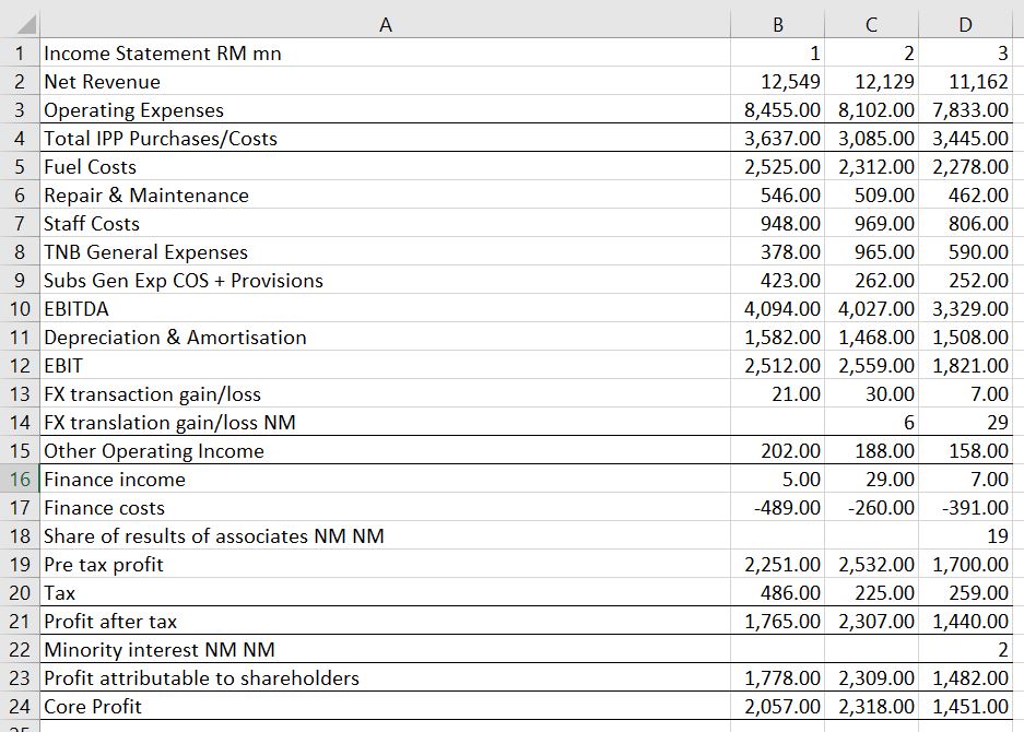
Lets say you have a bit of data that is arranged with periods across the top and items in each row. This could be any historic financial statement or any page from a financial model. The screen shot below is an example (that of course uses the read pdf from that you can download from another sheet). Now you would like to make a graph with a single line or multiple lines of each item in the chart. Note how all of the titles are in column A which makes things a lot easier.
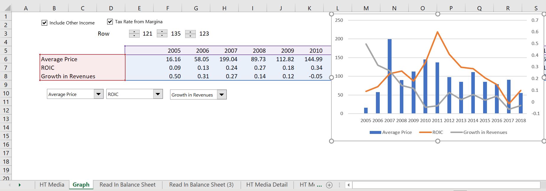
Once you get the file, all you do is to enter a row somewhere in the sheet across to the right of the detailed data or alternatively in a new sheet. Then use the index function WITH THE ENTIRE COLUMN using the row number for selecting the data, meaning you write something like INDEX(A:A,row number). Once you have done this for one column, copy the column to the right (it is a good idea to put the time line at the top of the new page and use SHIFT, CNTL, R to copy things to the right. After that, put in a spinner button and or a drop down box as illustrated on the screenshot below.
I think one of the most useful and quick things to do with a whole lot of data (for example a set of historic financial statements) is to use the INDEX function to graph all of the items on a sheet. All you have to do is to use a code number for the row of the sheet that you want graphed and then use the INDEX function with an entire column. You can then add a drop down box or a spinner box. The file below demonstrates how you can take just about any file and then add a drop down box (combo box) to graph any line on the page. You can also get a little fancier by using multiple columns for the name and avoiding blank rows. The technique and avoiding blank or title lines is a bit more difficult where you can include TRUE/FALSE switches on each line and then count the number with the MATCH function.
As long as you have the field name at the top as the years and the item, you could do this pretty easily in Power BI. One this one however, I think it is so easy to do with the INDEX function and a user form, you can do this in minutes. The problem with Power BI is that you may have to spend a lot of time fixing things to get the file ready for making graphs.
Making a Spinner Box that Skips Blank Rows so the Process Works with Blank Rows
If your financial statements or your financial model has blank rows, the process can not be artistic enough because there will be blanks in the drop-down box and because the spinner box will show a lot of blanks as you cycle up and down. You can solve this problem by attaching a macro to the spinner box. The macro can be designed so that when you hit a blank, the spinner box increments by an extra step. When you hit two blanks the spinner increases by two blanks and so forth. A file that has the spinner skip is available for you to download below.
Excel File with Spinner Box that Includes a Macro to Skip Blank Lines for Graphing
To implement this process, you need to define a couple of range names and attach the macro below to the spinner box. This involves:
- Step 1: Create a spinner box for the row number and a cell link
- Step 2: Put a range name called “Spinner” for the row number which is the cell link. Note that you can use a different range name, but then you must modify the macro that will be attached to the spinner box.
- Step 3: Compute some kind of total calculation using the INDEX function to test when an entire row is zero. You can use the INDIRECT function with INDEX and SUM as illustrated below. You can also test the title or something else that is zero when a blank line is hit.
- Step 4: Put a range name called “Output” in the total line from Step 3. As with the “Spinner” range name, you can use a different range name, but you must then change the macro.
- Step 5: Attach the macro below to the spinner box by right clicking on the spinner box.
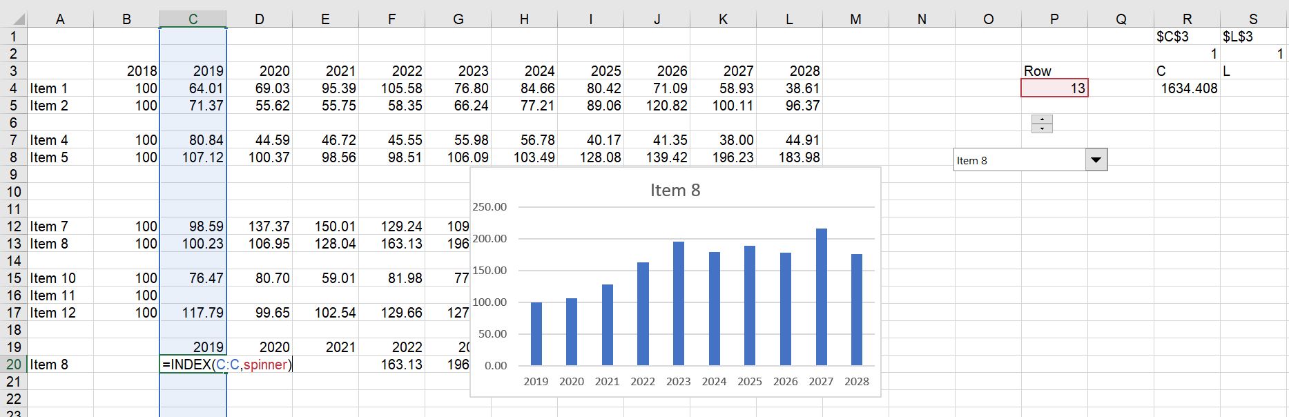
The screen shot below demonstrates the issue. There are a few blanks in the rows and the graph at the bottom uses the INDEX function. The spinner box shown on the screen shot is attached to a macro the skips rows which are blank.
The code that you can add to the spinner box is demonstrated below. You can download the file with this code or you can just copy the code below into your sheet (press the ALT F8) to get a list of macros. Then jut type in some new name like Stormy. Then, press the edit button to see the VBA code. Finally, just copy this code below to your code. When you use the code below, make sure you have the correct spinner box. You can right click on the spinner box and select the assign macro option. If it says something other than the Spinner1_Change, then adjust the title of the subroutine. Also make absolutely sure that you have the name OUTPUT and SPINNER defined. Finally, note that you can change the 1000 in the VBA code below to the maximum in your spinner box. This protects the spinner box from looping at the end.
Define the Range “Spinner”
Define the Range “Output” as the total
Public last_spinner As Single ' Needs to be public or will forget


Public last_spinner, current_spinner, count_skip As Single ' Needs to be public or will forget

Sub Spinner1_Change()

' Need two range names -- for the spinner and the sum of the output

application.displayalerts = false
application.screenupdating = false
current_spinner = Range("spinner")

re_start:

If Range("output") = 0 Then
If last_spinner < Range("spinner") Then

Range("spinner") = Range("spinner") + 1

count_skip = count_skip + 1

If Range("spinner") > 1000 Then
Range("spinner") = WorksheetFunction.Max(current_spinner - count_skip, 1)
End
End If
End If
If last_spinner > Range("spinner") Then
Range("spinner") = Range("spinner") - 1
End If
End If

If Range("output") = 0 Then
' MsgBox " Last spinner " & last_spinner & " spinner " & Range("spinner")
GoTo re_start: ' testing for multiple blank rows
End If

last_spinner = Range("spinner")

End Sub
Video Explanations