If you want multiple series options to put on a graph, you can add check boxes instead of using the list box. This page demonstrates how you can copy a whole bunch of check boxes and attach each check box to a TRUE/FALSE switch. With the multiple check box macros you can create graphs that find only the check boxes that have an associated with TRUE.
The most difficult thing about this is copying the check boxes when you may have more than 100 different possible selections. To do this I have make a macro in the file available for downloading below. It is not perfect and you have to be careful when operating it. The first step is to copy the check boxes and make sure that you have new numbers for the check box (that you can find with looking at a macro as demonstrated below). You cannot do this with manual calculation. After copying the checkbox you can run the macro with SHIFT, CNTL, E. As with other macros, save your file before running the macro.
Using the Attach Check Box Macro
To attach a whole bunch of check boxes, you can copy a lot of check boxes and then use the TRUE or FALSE created by the check boxes to count the number of selections. This process of attaching the TRUE/FALSE is illustrated in the screen shots below. When you open the file, the following appears and the SHIFT, CNLT, E macro that attaches TRUE/FALSE is implemented.

Now say that you have list of stock prices, countries, accounts or anything else that you want to graph in a flexible manner with check boxes. I have used the Sun Edison (bankruptcy) example as illustrated in the screen shot below. In this example we will make a graph of any of the items in the income statement with multiple check boxes. Using the SHIFT, CNTL, E, the process should just take minutes.

The file with the completed example is available for download by pressing the button below. The completed file has a number of check boxes whereby you can graph any of the items.
Sun Edison Bankruptcy Case Study with Example of how to Use Multiple Check Boxes and Flexible Graphs
With the attach check boxes file open, the next step is to make one check box and one TRUE false that can be copied downward. This is illustrated in the screenshot below.

You can then copy the TRUE and the check box down. Then find the number of the check box by right clicking and assigning a macro (do not attach a macro unless you want to; this is just to find the check box number that will be incremented. Note that in the example, the number of the check box is 1.

Once you have copied the check boxes and found the number, you can run the SHIFT, CNTL, E function. This function needs the start row and the end row as well as the check box number and the row for the TRUE/FALSE. The screenshot below shows what will come up after you run the macro. When you get the screen, fill in the row start and row end as well as the check box number.

After you have run the macro, the check boxes should be each attached to a separate TRUE/FALSE. You should try to press different check boxes and see if the process really works. After you have the check boxes you can move to the next step and make the graphs.

Process of Using Multiple Check Boxes to Create a Flexible Graph
Since you know that TRUE is 1 and FALSE is zero, you can create a column that counts the trues by adding the check boxes that are counted. This counter can then be matched against a counter variable to find the items that have been checked. You add a separate counter (you can use ALT, E, I, S) and then apply the MATCH function to find the number of the selection. Finally, use the INDEX function to put the items that are checked at the top. This process is illustrated below from the comprehensive stock price file. This process is illustrated in the series of screen shots below. The first screen shot simply shows how to accumulate the number of TRUES by making a cumulative counter.

The next screen shot demonstrates how to use the accumulation counter and the MATCH function to find the appropriate row with the first and second and third TRUE etc. This is illustrated in the screenshot below.

As usual, after the MATCH you can use the INDEX function. The MATCH and INDEX functions can then be copied and used to make the graph. The INDEX function is illustrated in the final screen shot below.

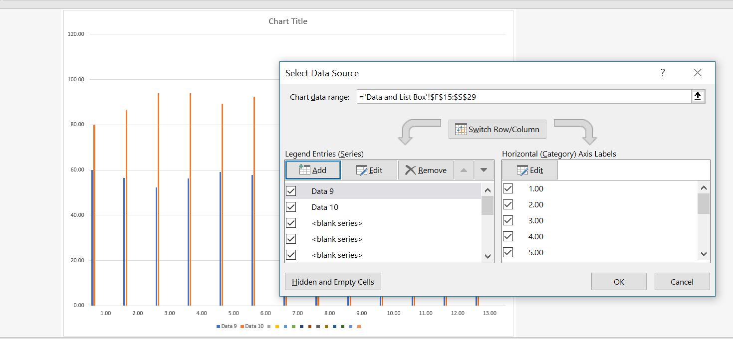
Assuring that NA and Blanks are not on the Legend of the Graph
It is tricky to put a legend without #NA in the graphs after you have made the flexible graphs with the multiple check boxes. You can make a dynamic range with the OFFSET function (by putting in the number of rows and columns in the height and width option). To make the range name stay in the graph, or more precisely, change the graph when the listbox changes, you can make a little VBA code. This re-does the data source when you change the list box.
A file that includes the VBA code to create flexible charts with legends that change is available for download by clicking on the button below. In this file you can press the CNTL and F3 sequence to see the dynamic range name. This range name (graph_data) changes when the list box changes and different numbers of graphs are selected. When you click the box named “adjust legend”, the legend should change.
The VBA code that allows you to remove the blanks or the #NA’s from the legend is shown below. You can either code into the macro for the listbox or you can include a separate macro. Of course, you need to find the name of your chart and adjust the macro accordingly.
Sub Adjust_legend()
'
'
 current_cell = ActiveCell.Address

 ActiveSheet.ChartObjects("Chart 8").Activate

ActiveChart.SetSourceData Source:=Range("graph_data")

 Range(current_cell).Activate

End Sub
Video Explanation of Multiple Check-Boxes to Make Flexible Graphs
The process for creating check boxes is illustrated below from the template file named “Attach Multiple Check boxes.” The file associated with this video is the file that you can download above. There may have been a couple of improvements in the file since I first made the video.
[wonderplugin_video iframe=”https://www.youtube.com/watch?v=ZCWjKogO6eA” videowidth=600 videoheight=400 keepaspectratio=1 videocss=”position:relative;display:block;background-color:#000;overflow:hidden;max-width:100%;margin:0 auto;” playbutton=”http://edbodmer.com/wp-content/plugins/wonderplugin-video-embed/engine/playvideo-64-64-0.png”]
VBA Code for Attaching Check Boxes
The VBA code that attached the list boxes is presented below.
.
Public Sub Auto_Open()
'
' Make a menu with an add-in
'
 Application.OnKey "^E", "attach_check"

Application.StatusBar = "SHIFT,CNTL,E --> Create Check Box Links "

start_row = 4
end_row = 33
start_box = 1
col_link_letter = "F"

End Sub

Sub auto_close()

 Application.OnKey "^E"
End Sub


Sub attach_check()

UserForm1.TextBox1 = start_row
UserForm1.TextBox2 = end_row
UserForm1.TextBox3 = start_box
UserForm1.TextBox4 = col_link_letter

UserForm1.Show

start_row = Val(UserForm1.TextBox1)
end_row = Val(UserForm1.TextBox2)
start_box = Val(UserForm1.TextBox3)
col_link_letter = UserForm1.TextBox4

current_sheet_name = ActiveSheet.Name
sheet_name = "'" & current_sheet_name & "'!"
Count = 0

start_box = start_box
range_box = "Check Box " & start_box
For Row = start_row To end_row
   range_box = "Check Box " & start_box + Count
   range_name = col_check_letter & Row
   On Error GoTo make_sure_copy:
   ActiveSheet.Shapes.Range(Array(range_box)).Select
   On Error GoTo 0
   link_name = sheet_name & col_link_letter & Row
   Application.CutCopyMode = False
   With Selection
     .Value = xlOn
     .LinkedCell = link_name
     .Display3DShading = False
   End With
 Count = Count + 1
Next Row

Exit Sub
exitsub:
MsgBox " make sure you have the correct checkbox number:"
Exit Sub
make_sure_copy:
MsgBox " Make Sure you Copy and Calculation is on when you copy "
End Sub

.