This page is an introductory page to sub-menus that address more advanced issues associated with debt sculpting. The advanced issues include multiple debt issues, curved sculpting, DSRA changes and scuplting and other issues. You can go to other menus too find these issues. In general, after you have structured the model without debt and without circular references, you can begin to enter debt into the model. If you are structuring the debt — finding the debt size, computing different debt repayments, trying different methods of funding debt, putting in different cash flow sweeps or even changing fees and interest rates, you will most probably run into circular references. From a theoretical perspective the circular issue arises because the model drives the negotiation of debt terms, but the debt terms drive the model. For example, the model drives the amount of Interest During Construction and is necessary to evaluate the total debt. But the total debt percent is driven the term sheet. In explaining the structure of debt draws, debt repayments and interest in a project finance model I suggest that you create the model without circular references. The file that you can download below that accompanies the discussion does not have circular references — I just left blanks for things like the DSRA flows, the accumulated IDC and the tax effect of interest on CFADS.

Playlist on Sculpting Issues
If you are in the mood for torture or maybe if you are having trouble sleeping, you can look through the sculpting playlist. I have put together various sculpting videos that I have made over the years. I have tried to put the more basic videos first (with the exception of the very first). The videos all apply the fundamental formula that the PV of debt service over the repayment period is equal to the debt size at the beginning of the repayment period (i.e. the period just prior to the commercial operation date). Over time I have learnt more about sculpting issues that can involve curved DSCR’s, multiple debt issues, incorporation of on-going fees, alternative debt sizing options, complex income taxes and computation of DSRA moves as part of the CFADS. I hope I have covered a lot of these issues in the videos. As with other items, you can always send me an email at edwardbodmer@gmail.com.
.
.
.
Setting-up Debt Assumptions and Debt Schedules
I have taken a long time to add the debt issues to this A-Z lesson. When you add debt to a project finance model you will run into circular reference issues. These circular references come from both funding and and repayment issues. In working through the various debt structure subjects I show how to set-up the model without circular references. Then, in the next section, I show you how to use UDF’s which will enable you to check your work and to create nice flexible dashboards. I hope you will stop being a copy and paster in all areas of your life.
Before starting to go though the various mechanical debt financing subjects, you should download the two files that I am using for this exercise. I am sorry, but these files are different from the files above as I have tried to focus on tricky debt sizing issues. These file connected to the buttons below use the case of a wind farm with different debt sizing possibilities (from P99, P50 and debt to capital), multiple debt sizing issues and multiple re-financing possibilities. You can download the files that are used for completing exercises and a completed version of the files by clicking on the buttons below.
Videos on Debt Structuring
Structure of Inputs and Assumptions
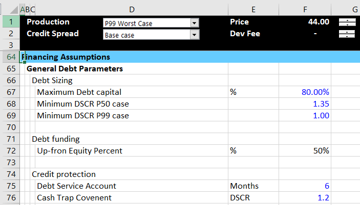
The manner in which you can set-up assumptions when you have multiple debt issues is illustrated in the screenshot below. You should understand that some parameters apply to all debt issues. You cannot have more than one overall debt service coverage ratio (you can have a senior DSCR and a total DSCR — not a subordinated DSCR). You cannot not have more than one overall debt to capital ratio. The DSRA that protects lenders is generally on the overall debt service. Other parameters such as the interest rate, the debt tenure and the repayment pattern of debt can be defined on an individual debt issue basis. The screenshot below illustrates how you can set up the debt assumptions with one debt issue. The first screenshot illustrates how there can be multiple overall debt sizing constraints and how the the funding of debt is driven by a parameter for up-front equity funding.
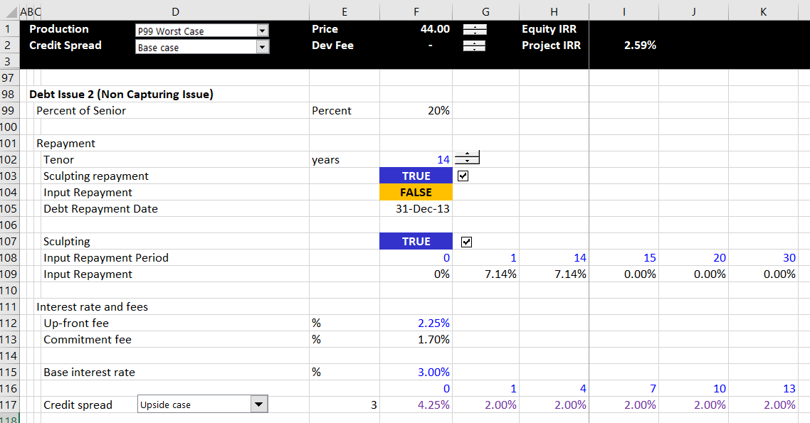
The screenshot below illustrates inputs and assumptions that should be input on an issue by issue basis. The first input is for the percent of the total debt that is represented by the debt issue. I have labeled this issue as a not capture issue. This is because if there are multiple debt issues and sculpting, there must be one issue that captures the rest of the debt service and assures that the total debt service is met. I find the whole idea of sculpting for multiple debt issues complex and there I have included a separate page that deals with the multiple debt issue sculpting subject. The debt tenure is entered by issue and if the debt with the longest tenure should generally be the debt capture issue. You can enter a grace period near the tenure and you can put in specific dates for the start and end of the repayment. Note that I have used the generic macros file to colour the various things (please just try this). As with my general philosophy I hope you keep the structuring of the debt issues consistent — the size, the funding, the repayment, the interest rate and fee and the protections.
Structure of Debt Size and Summary Sources and Uses of Funds
Once the inputs are established, I suggest structuring the whole model without circular references, meaning that you enter the titles and make various calculations. Structuring the whole model without the circular references means that you can leave some items like IDC in the periodic sources and uses funds blank. You may also make some errors on purpose like not subtracting taxes in computing CFADS In other cases, like for the debt IRR, you may want to just enter a fixed number.
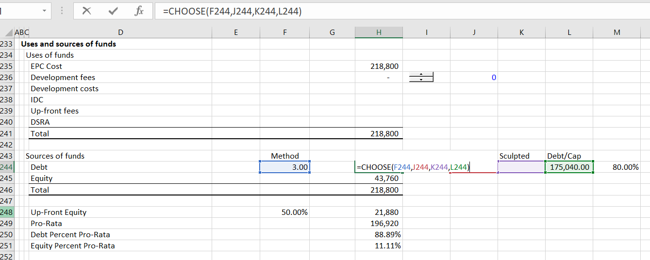
Now let’s move to the modelling of debt size, debt funding, debt repayment, interest and fee costs, and credit protections. One way or another I suggest that you put in a summary sources and uses of funds statement with the total amount over the construction period. If you are setting up your model, you will not be able to enter the IDC (I Don’t Care, or interest during construction), the DSRA, and the fees. You will generally also not be able to enter the amount of the debt. But just enter a placeholder for the debt and leave the IDC, DSRA and fees blank. Then your summary sources and uses of funds should look something like the screenshot below. This is the first step of the analysis and this is related to the debt sizing. Note how I have put options for debt sizing from debt to capital or from input debt or from sculpting to the right of the debt amount and these are not yet filled-in. The fact that these items are not entered yet should be giving you anxiety about circular references. When you have to go downstairs to find stuff, circular references are an issue.
Cash Flow Statement Number 1 – Sources and Uses During Construction
Now let’s turn to funding of the debt during construction given the amount of debt and equity from the summary sources and uses of funds statement. I am using the Hedieh method of entering the equity up-front as an input variable. I think this is brilliant. If you want everything to be pro-rata, you can enter zero as the equity up-front percent. If you want to use all up-front funding, you can enter 100% for the input. Of course you can enter anything between. Given this input for which I used 50%, which implies that some of the funding is equity up-front and some is pro-rata. In the screenshot above, in the section below the sources and uses of funds I have computed the percent of funding that comes from pro-rata debt and pro-rata equity. To make this calculation compute the 50% of equity up-front first. Then you can derive the total pro-rata funding. The debt percent of pro-rata is the total debt divided by the pro-rata funding and the equity is the remainder.
Once you have the pro-rata percentages you can enter the sources and uses funds statement on a period by period basis. You should think of this as a cash flow statement before COD. Before COD there is no EBITDA and no cash inflow, so everything is about finding cash to fund the various needs which include capital expenditures and can include IDC, fees, DSRA funding, Development costs, Development fees and so forth. An example of cash flow statement before COD (the sources and uses of funds) is illustrated in the screenshot below. Note that the numbers are not filled-in. This is again because of the circular reference nightmare.
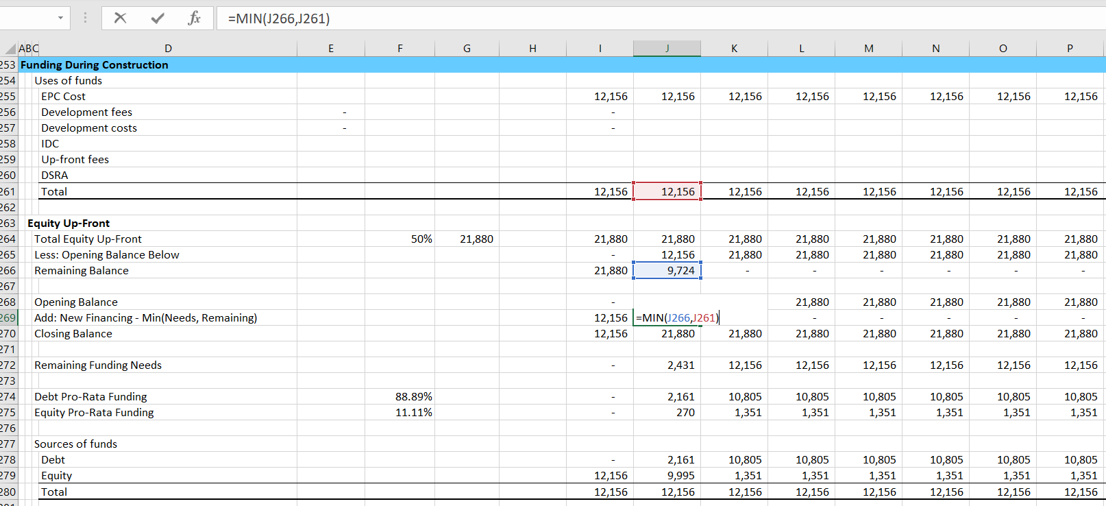
To compute either equity-up front or pro-rata funding, you can begin by evaluating the equity up-front. I have seen many ways to do this, but I start by computing the amount of remaining equity that can be used to fund equity that will be used in the MIN function. I do this by first computing the total equity commitment an then subtract the amount of equity already used which is the opening balance. Then, I compute the opening and closing balance of the equity. The amount of funding is computed with the MIN function where you compute the minimum of the funding needs or the remaining equity.
Equity Funding = MIN(Remaining Funding, Cash Needs)
Structure of Debt Schedules with Multiple Issues
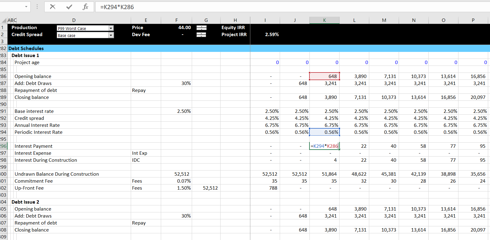
After the first cash flow statement — the sources and uses of funds by period — is established, you can enter the debt schedule. The debt schedule simply presents the opening balance, additions and closing balance. I cannot imagine a project finance model that does not have a debt schedule. In the example below, I have left out the repayment which is addressed in the next section. As you can see, the debt schedule also includes interest rates and fees with a separation of interest between IDC and interest expense. This is pretty standard with maybe the exception that the debt draws are computed from the percent of total debt that is gathered from the sources and uses of funds statement.
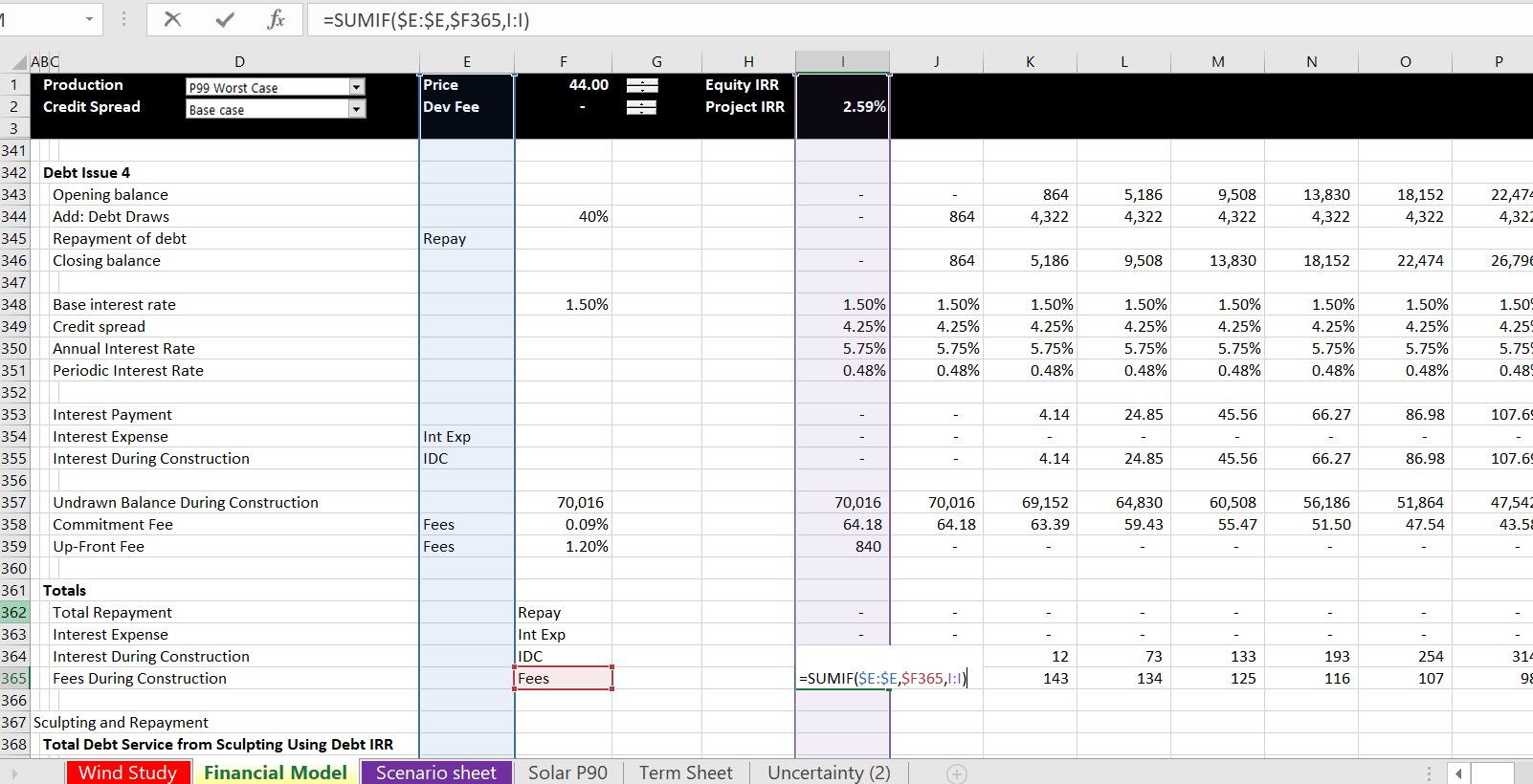
I have also included a screenshot with the summary of all of the debt issues below. This just adds up all of the interest cost and the IDC and the fees using a SUMIF function. Of course I apply the lazy principle and use the SUMIF with the entire columns of data. As with the debt schedule, this is just a long and painful process. Note that after the total fees and the total IDC is computed, I have not placed the amount in the sources and uses of funds. When you put the IDC and the fees into the sources and uses of funds, a dreaded circular reference occurs.
Structure of Repayment with Multiple Sculpting
In this A-Z exercise I have included repayment schedules where multiple debt issues are used to sculpt. On another page in the advanced project finance section I explain this process in detail. Please note that you can compute this by temporarily pretending that CFADS is the same as EBITDA. You will change this when you implement the UDF below. In brief, if you want multiple sculpted issues that produce both the target DSCR and the correct allocation of debt, you can do the following:
1. Compute the aggregate amount of debt with the aggregate CFADS using a debt IRR. To compute the debt IRR you will have a circular reference because the amount of aggregate debt is used to apportion the debt, compute debt service and ultimately arrive at the debt IRR itself.
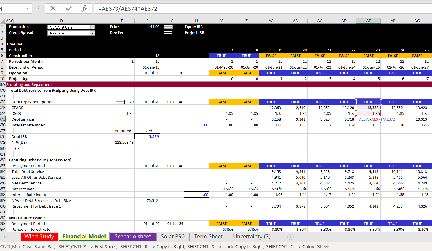
2. Compute the debt service for the capturing debt issue. This capturing debt issue is computed similar to the aggregate debt, but the interest rate on the debt issue is used and the debt service on the other issues are subtracted. The screenshot below illustrates computation of the capturing debt issue and the aggregate debt.
3. Compute the LLCR for the non-capture debt issues. Do this by first computing the debt balance associated with the debt issue where the balance is the total amount of the debt from the NPV of the aggregate debt service in step 1. This is multiplied by the target debt percent. Once you have the debt balance for the non-captured issues, this is the denominator of the LLCR used for sculpting. The numerator is the PV of CFADS at the relevant interest rate. The LLCR that is shown in the second screenshot is computed using the formula:
LLCR = NPV(CFADS)/Debt from Aggregate Debt Balance * Percent Debt
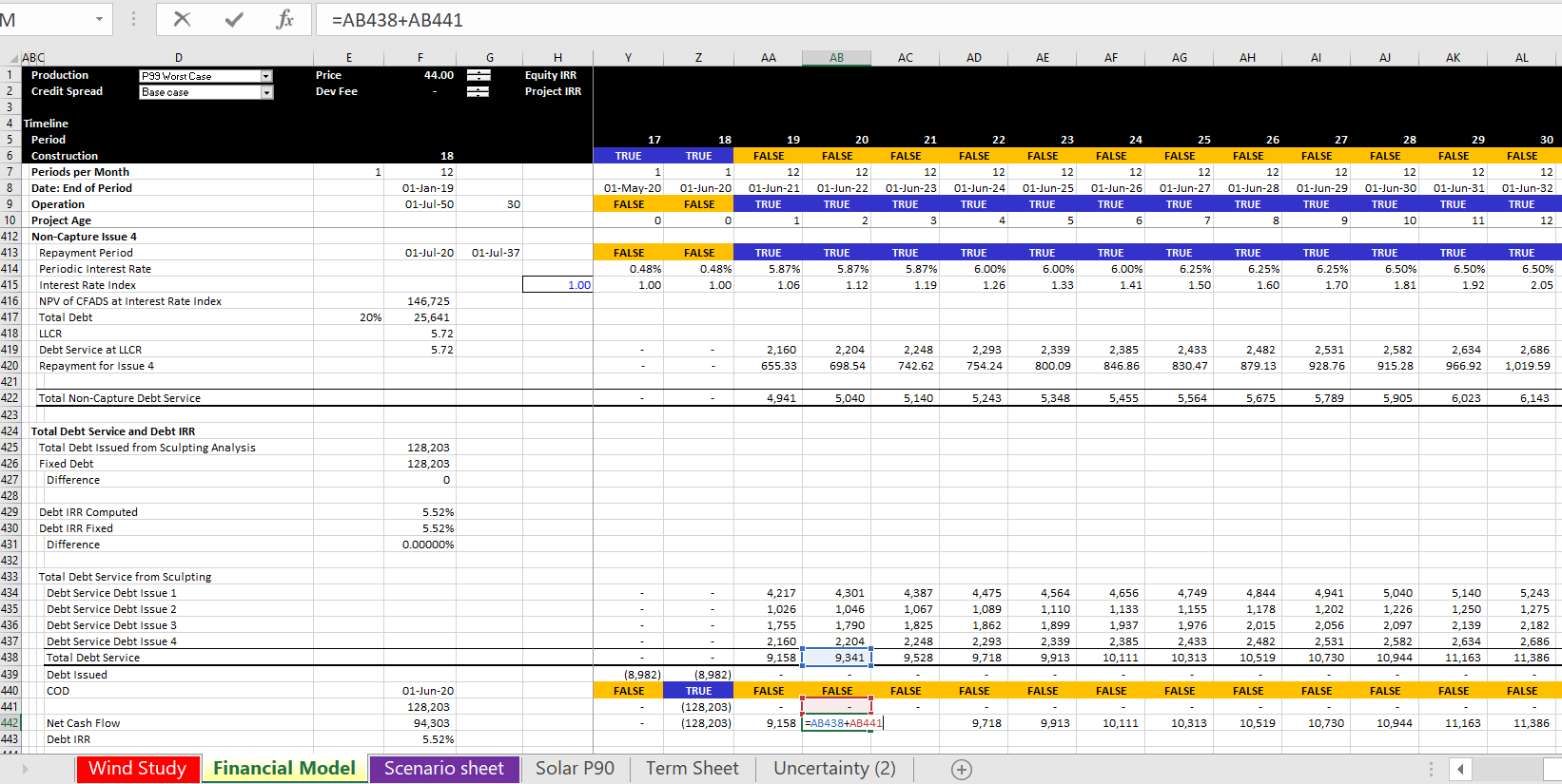
4. The final part involves computing the debt IRR from the total debt service. To calculate this, add the debt service from the different issues. Then put the total debt issued at the COD as the negative investment. With the cash flow on debt, compute the debt IRR. Note that there are two circular references from this process. The first is the IRR and the second is the debt balance. We are setting-up the schedules so do not worry about these yet.