Sculpting – Edward Bodmer – Project and Corporate Finance

This page explains how you can construct a project finance model that includes sculpting where there are multiple debt issues and one or more of the debt issues is used for sculpting. In the case where there is one debt issue with a balloon payment and sculpting, the balloon payment can be split from the rest of the debt issue and then be modelled as a two different debt issues, one of which operates as the sculpted debt issue. The balloon issues is almost identical to the issue of min-perms. When there are multiple debt issues all of which are sculpted, allocation of the debt to different issues with different interest rates and different debt tenors, the calculations are more complex. This type of situation with multiple debt issues that are sculpted can occur when there is an issue from a development finance institution as well as an issue from a private bank. The private bank may often be sculpted in the same manner as the DFI, but have a short tenure.

Instructions for Downloading Files with Macros

Formulas and mechanical techniques for a basic case of sculpting with two debt issues are included in the file that has various different exercises. You can file this file on the google drive in the Project Finance Section under exercises and then Section D for the Sculpting course. The file is also available for download by pressing the button below. This file does not address balloon payments which are a little more difficult because the size of the balloon payment affects the DSCR on the non-balloon portion which in turn affects the size of the balloon payment and you have a good old fashioned circular reference.

Excel File with Focused Separate Sculpting Exercises and Analysis from Basic Debt Sizing to Advanced with VBA

Formulas for Multiple Debt Issues where There is Only One Sculpted Debt Issue

Very often, there is more than one debt issue in project finance transactions. When there are multiple debt issues and one of the debt issues (defined as Last or the sculpting capture issue) is used for sculpting. In this case the basic formula can be adjusted and the process if straightforward. You can start with the DSCR formula and derived the debt service for the last formula. Note that if you are sculpting two debt facilities at the same time and these facilities have different interest rates and different tenures, then the process is difficult because for the NPV formula you need a common interest rate.

You can use the following couple of equations to resolve the case where there are multiple debt facilities and repayment for one of the debt issues is determined from sculpting. For the equations, the term Other DS is the debt issue on the non-sculpted issue (which could be balloon portion of the sculpted issue). The term Sculpted Issue DS represents the debt service for the debt issue where repayments are determined from sculpting.

DSCR = CFADS/(Other DS + Sculpted Issue DS)

Other DS + Sculpted Issue DS = CFADS/DSCR

Sculpted Issue DS = CFADS/DSCR – Other DS

The modelling of multiple debt issues using the sculpting exercise file that you can download above is illustrated in the screenshot below. In this example there are three debt issues, the last one of which has sculpted repayments driven by sculpting from CFADS. If the debt is separated in this manner, developing sculpting is pretty easy. The problem comes when the first issue is a function of the sculpting itself. This is the issue with balloon payment.

Modelling Balloon Payments or Mini-Perm with Sculpted Debt Issues

If there is a bullet repayment at the end of the debt tenure (say 15% of the repayment), then the bullet repayment can be considered a separate debt facility. So, if the bullet repayment is 15% then the PV of the repayment is a separate facility with interest over time etc. The NPV of the remaining debt should subtract the interest and the repayment on this separate debt. Since the bullet repayment affects the amount of sculpting and the NPV of the debt multiplied by 15% drives the bullet repayment, the bullet repayment causes a circular reference.

You can see more details of how to model balloon payments in a separate section of the website. The button below provides a link to the balloon repayment section which includes VBA necessary to make the models.

Go to the Website Page that Describes the Modelling of Balloon Payments and Includes VBA

Excel File with Focused Separate Sculpting Exercises and Analysis from Basic Debt Sizing to Advanced with VBA

Formulas for Multiple Debt Issues where There is Only One Sculpted Debt Issue

DSCR = CFADS/(Other DS + Sculpted Issue DS)

Other DS + Sculpted Issue DS = CFADS/DSCR

Sculpted Issue DS = CFADS/DSCR – Other DS

Modelling Balloon Payments or Mini-Perm with Sculpted Debt Issues

Go to the Website Page that Describes the Modelling of Balloon Payments and Includes VBA

If you are in the mood for torture or maybe if you are having trouble sleeping, you can look through the sculpting playlist. I have put together various sculpting videos that I have made over the years. I have tried to put the more basic videos first (with the exception of the very first). The videos all apply the fundamental formula that the PV of debt service over the repayment period is equal to the debt size at the beginning of the repayment period (i.e. the period just prior to the commercial operation date). Over time I have learnt more about sculpting issues that can involve curved DSCR’s, multiple debt issues, incorporation of on-going fees, alternative debt sizing options, complex income taxes and computation of DSRA moves as part of the CFADS. I hope I have covered a lot of these issues in the videos. As with other items, you can always send me an email at edwardbodmer@gmail.com.

Modelling Multiple Debt Issues All with Sculpted Repayment with Different Tenures and Different Interest Rates Using Capture and Non-Capture Issues

This section moves from fairly basic issues to a difficult issue where you are not given repayment on the non-sculpted debt issues, but you have to compute sculpted repayment on many debt issues. The mechanics of computing multiple sculpting is more difficult than where you have one sculpted debt issue and one non-sculpted issue as in the case of the balloon payment. As shown above, the modelling of sculpting is not all that difficult where only one of the debt issues is sculpted. You can use the formula to derive the sculpting by using the following formula:

Sculpted Issue DS = CFADS/DSCR – Other DS

If other debt issues are sculpted, this formula does not work in a simple manner. In this section I explain how you can compute sculpted debt repayments and debt service when you have multiple debt issues with different terms (tenures and interest rates). I have put together a file that includes issues of calculating debt service for multiple debt issues in the file below.

Excel File with Demonstration of How to Compute Sculpting for Multiple Debt Issues with Different Tenures and Interest

With multiple debt issues, I define one debt issue — the issue with the longest tenure — as the capture debt issue. Other debt issues are defined as the non-capture debt issues. The rule to computed sculpted debt repayment where you have multiple debt issues is the following:

Compute the overall debt IRR using all of the sculpted debt issues when you compute the NPV of the CFADS.
Compute the LLCR for the non-sculpted debt issues using the interest rate of the debt issue, the tenure of the debt issue and the CFADS to calculate the numerator. The denominator of the LLCR is the amount of debt which is the NPV of the total debt issue multiplied by the target debt percent.
Compute the debt service of the captured debt issue using the target DSCR for overall cash flow and the debt service of all of the other non-captured debt issues. This applies the formula DS = CFADS/DSCR – Non-capture Debt Service.
Compute the IRR using the net debt cash flow that includes the total amount of the debt and the total amount of the debt service.

1. Simple Allocation of Cash Flow Method to Compute Sculpted Balances

To introduce the issue I have created a simple example with three debt issues. Each issue has a different debt tenure and a different interest rate. Each issue also has a target amount as percent of the total debt. This set-up of the sculpted debt inputs is shown in the screenshot below. If there is a loan from a development financial institution, this type of situation with multiple debt issues that are sculpted can occur. If there is also a non DFI, the non DFI may have a shorter tenure and a higher interest rate. Note that the last debt issue in the screenshot has a tenure of 14 years while the first issue has a tenure of 8 years.

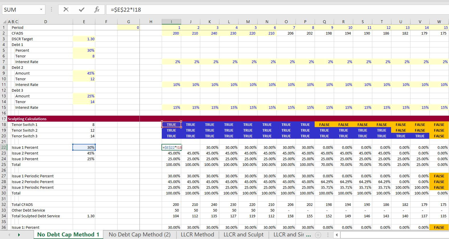
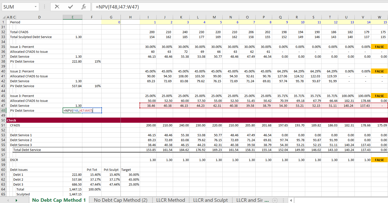
In the above screenshot I entered the target sculpting for each debt issue. This had to be computed twice to recognise that after the first debt is finished, the percentages will change. Ultimately, when there is only one debt issue outstanding, all of the cash flow is allocated to that issue. These percentages are applied to the CFADS and then the sculpting is made with the normal NPV formula. The calculation of sculpting from the allocated CFADS to each issue is shown in the screenshot below. The NPV of the debt service gives you the total amount of debt as usual. If the interest rate is lower the NPV of the debt is higher. If the tenure is longer the NPV is higher. All of this means that the target percentages do not equal the final debt balance percentages. This is demonstrated at the bottom of the page. On the table at the bottom of the page, the target percentages computed from the NPV of debt service are very different from the target percentages.

2. LLCR Method to Allocate Sculpting for Multiple Debt Issues

I have described how you can compute sculpting if the debt balance is given. In this case you can use the formula to find the target DSCR to sculpt from a simulated LLCR. The formula is:

LLCR = PV(CFADS)/Debt

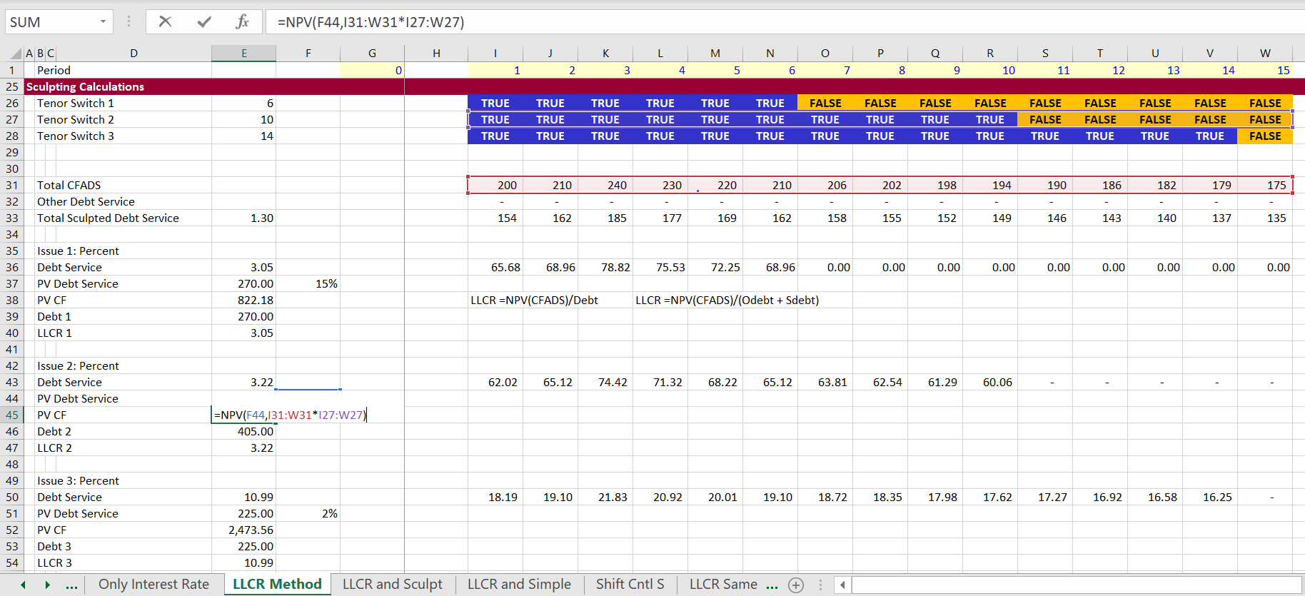
In the example below, the total debt is given as a fixed amount of 900 and it is allocated between three debt issues. For each issue, the PV of cash flow over the tenure of the debt is computed. Then, the total debt of 900 is allocated among the three issues. This defines the target amount of debt. The LLCR is computed for each issue from the PV of Cash Flow as well as the target amount of debt. This computation of the LLCR is illustrated in the screenshot below. The formula in the screenshot illustrates how you can put a formula (with TRUE/FALSE multiplied by the CFADS) into the NPV formula. Note that the LLCR is very high because the total cash flow is compared each separate debt issue.

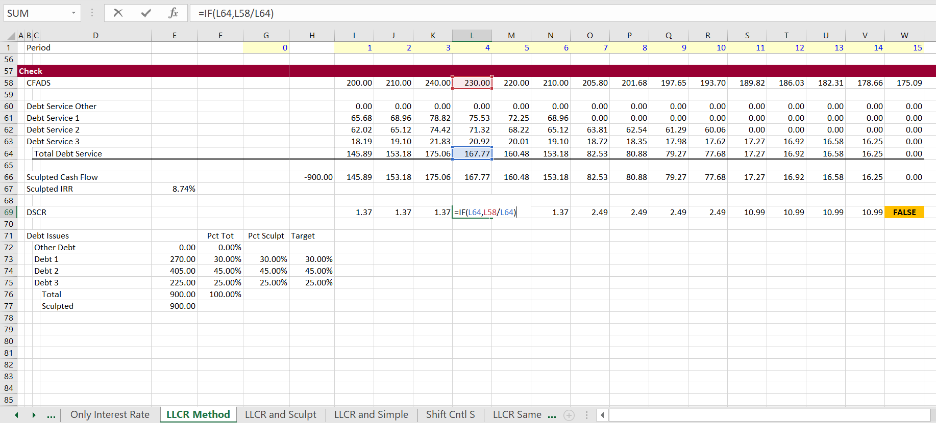
Results of the LLCR method are shown in the screenshot below. In this screenshot the good news is that the amount of debt is the target debt. But don’t get too happy. The very bad news is that the DSCR does not match either the LLCR on the overall debt or the target DSCR. Note that the DSCR begins at a level of 1.37. But after the first debt issue is finished, the DSCR increases to 2.49. Then, when only the last issue is outstanding, the DSCR is 10.99. If you allocate debt in this way the fact that the DSCR is not constant demonstrates that the method does not work.

3. LLCR on One Issue and Remainder Formula for Second Issue

The next method is getting a bit closer, but it still does not quite work. In a case with different interest rates and only two debt issues, you can reach both the target DSCR and the target percentages of debt. The method starts by establishing the overall debt size from the target DSCR. The debt size is derived by computing the NPV just like in any of the debt sizing cases. This interest rate is used in the formula Debt = NPV(Debt IRR, Debt Service) where Debt Service = CFADS/Target DSCR. But to compute the debt size, you need a discount rate. The discount rate is the overall IRR on debt is computed from evaluating the total amount of debt versus the debt service from all of the debt issues.

The method of establishing the LLCR fror one issue and using the debt service formula for the second issue works when the tenure is the same for both issues because of a circular reference problem. The screenshot below illustrates the approach. The first debt issue is computed with the LLCR using the method discussed in the prior section. The PV of cash flow is computed and then the LLCR is derived from the target amount of the debt: LLCR = PV Cash/Debt. Using this LLCR to compute debt service produces debt service for the first debt issue and it also yields the target debt size for the first issue. For the second issue, the formula for debt service of is DS = CFADS/DSCR – Other DS, where the Other DS includes the debt service from the first debt issue. I label this debt issue as the capturing debt issue. When you compute the NPV of this cash flow for the second issue, you get the same amount as the target debt percent multiplied by the total debt.

A complexity with this method is that works from the IRR on the overall debt. This is needed because the IRR on the debt that is used for sculpting. But the IRR on debt cannot be computing until the debt issues are evaluated. This causes a circular reference which will be discussed in detail below. This is shown in the second screenshot below.

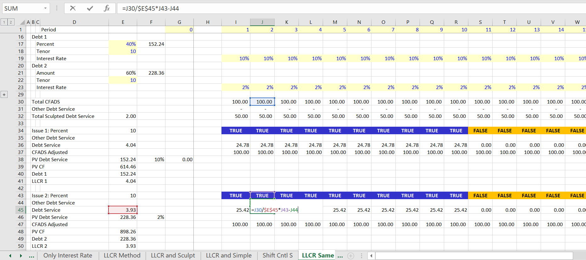
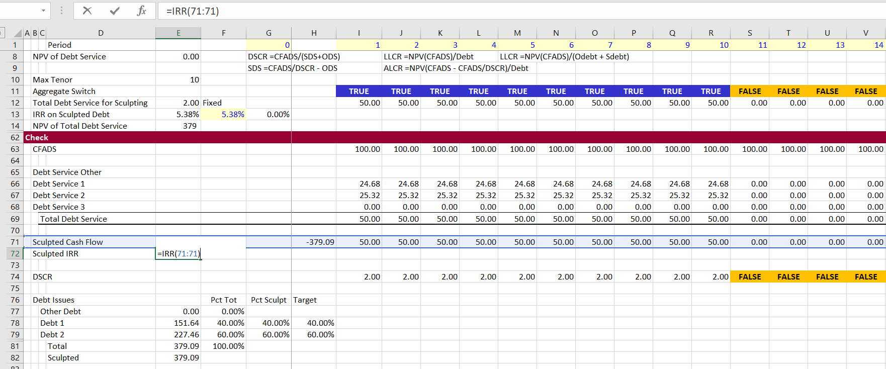
The next screenshot demonstrates the results of this combination of LLCR and formula method. In this method, the target DSCR of 2.0 is achieved and the target debt amounts for the two issues are also achieved as shown on the bottom of the screenshot. To make this computation work, the debt IRR is computed from the debt service of the two debt issues. This IRR is 5.38%. But the IRR is not known until the debt service of the two issues is computed. The IRR is copied and pasted into the calculation for the NPV of overall debt service.

Using SUMIF to Aggregate Interest Expense, IDC, Repayment and Balance

4. LLCR on and Maximum Tenure with Circular Resolution

The multiple sculpting issue can be solved when you set-up the analysis to first establish which issue has the longest tenure. This debt issue with the longest debt tenure is labeled the capturing debt issue as in the last section. Once the maximum debt tenure is established, the process of computing sculpting with multiple debt issues involves the following steps:

Step 1: Compute the maximum debt tenure from the debt tenure of all of the issues

Step 2: Insert a discount rate and compute the total debt from the present value of the debt service derived from the target DSCR. The discount rate is the debt IRR

Step 3: Compute that size of each debt issue from the given percent of debt. This is shown in the screenshot below.

Step 4: For the non-capture debt issues, compute the present value of cash flow at the interest rate of the debt issue and account for the tenure of the debt. This is shown in the screenshot below.

Step 5: For the non capturing debt issues, compute the LLCR in order to derive the debt service for the different debt issues. The LLCR is computed from target amount of the debt and the present value of the cash flow.

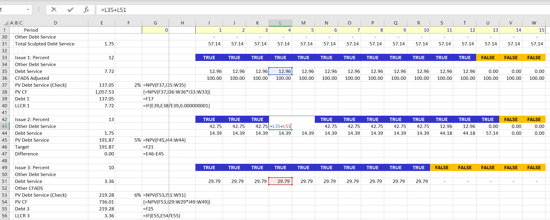
Step 6: Compute the debt service for the non-capture debt issues using the LLCR and the debt tenure.

Step 7: For the capture debt issue, the debt service is computed as DS = CFADS/Target DSCR – Other Debt Service; where the other debt service in the formula includes debt service from the sculpted issues that are not the capturing debt issue. This is illustrated in the screenshot above.

Results of a case with changing interest rates and also a debt issue with non-sculpted debt is shown in the screenshot below. For this case, the non-sculpted debt service is included in the subtraction from the capture debt issue. To implement the changing interest rate, use the SUMPRODUCT function with and interest rate index.

Developing a UDF to Resolve the Debt IRR and the Debt Size with Multiple Debt Issues

Set-up the Structure of the UDF

The first excerpt below demonstrates how to set-up a UDF where the output will go to more than one cell and be an array function. To do this, you begin by defining the function as a Variant as shown in the function definition below. Then I define an output array. The dimensions of the array are the row first and the column second. The array dimensions just have to be large enough to cover the total number of rows and columns that will be created by the function. As shown in the example, some sort of definition must be made of the output array. Finally, the name of the function is assigned to output array. The Option base 1 is defined at the very top of the page. When you use Option Base 1 the first row will be the item of the array with the number 1 rather than the number 0.

Option Base 1

Function mult_sculpt() As Variant

Dim output(10, 100) As Single

' PUT IN THE CODE AND DEFINE OUTPUT

output(1, 1) = debt_irr
output(2, 1) = debt_balance

mult_sculpt = output

End Function

.
.

Work Backwards

Once you have created the structure of the UDF program, begin at the end and start working backwards. In this case, the end is computing the debt IRR. The debt IRR is in turn computed from the debt cash flow which must be defined. Note that when you write the code, you can generally use excel functions with the WORKSHEETFUNCTION statement. After you start at the end, keep working backwards until you have defined all the equations that are needed.

.

Option Base 1

Function mult_sculpt() As Variant

Dim output(10, 100) As Single
Dim debt_cf(100) As Single

' Keep Going Backwards

debt_cf(i) = -debt_balance

For i = 2 To 40
   For k = 1 To 3
     debt_cf(i) = debt_cf(i) + debt_service(i, k)
   Next k
Next i

debt_irr = WorksheetFunction.IRR(debt_cf)

output(1, 1) = debt_irr
output(2, 1) = debt_balance

mult_sculpt = output

End Function

.

Continue to Work Backwards and Define Required Inputs

The next insert illustrates how to keep working backwards and compute the debt service for the different issues. You can make a loop that goes around the different debt issues and make the different calculation for the capture debt issue and the other debt issues. In the calculation for the captured debt issue, the CFADS and the target DSCR are necessary. These are inputs that will have to be read into the function. For the non-captured debt, the sum of the debt service is necessary.
.

Option Base 1

Function mult_sculpt(cfads,target_dscr) As Variant

Dim output(10, 100) As Single
Dim debt_cf(100), debt_balance_issue(10), debt_cf(10, 100), cfads(100), llcr(10), non_capture_ds(100) As Single

' Keep Going Backwards

capture_k = 2

For k = 1 To 3
   If k <> capture_k Then
      For i = 1 To 40
         debt_service(k, i) = cfads(i) / llcr(k)
         non_capture_ds(i) = non_capture_ds(i) + debt_service(k, i)
      Next i
   End If
Next k

For k = 1 To 3
   If k = capture_k Then
      For i = 1 To 40
         debt_service(k, i) = cfads(i) / target_dscr - non_capture_ds(i)
      Next i
   End If
Next k

debt_cf(i) = -debt_balance

For i = 2 To 40
   For k = 1 To 3
      debt_cf(i) = debt_cf(i) + debt_service(k, i)
   Next k
Next i

debt_irr = WorksheetFunction.IRR(debt_cf)

output(1, 1) = debt_irr
output(2, 1) = debt_balance

For i = 1 To 40
   output(3, i) = debt_cf(i)
Next i

mult_sculpt = output

End Function

Create and Iteration Loop for Circular Reference

After you have worked through the equations you can make an iteration loop. I am often lazy about this, but it is best to put in a loop that goes around until the circular reference is solved. When I am lazy I just use a simple FOR NEXT loop. But it is best to find one of the sources of circular reference. Then you can see when the difference between the current iteration and the last iteration for that variable declines to zero or almost zero. To do this you better make sure that the very first iteration does not go to zero.

Further Information and Learning: Request Resource Library (Free), Details About Courses

last_debt_balance = 999
debt_balance_difference = 999

Do While debt_balance_difference <> 0

last_debt_balance = debt_balance

' All the stuff

debt_balance_difference = last_debt_balance - debt_balance

.

Final Circular Resolution

.

Function mult_sculpt(cfads, target_dscr, target_pct1, tenure1, int_rate1, _
target_pct2, tenure2, int_rate2, target_pct3, tenure3, int_rate3) As Variant

Dim output(10, 100) As Single
Dim debt_cf(100), cfads1(100), debt_balance_issue(10), llcr(10), non_capture_ds(100) As Single
Dim debt_service(10, 100), debt_service_capture(100), target_pct(10), tenure(10), int_rate(10) As Single
Dim pv_cash_flow(10), cfads_issue(100), overall_debt_service(100) As Single

' Keep Going Backwards

capture_k = 2

tenure(1) = tenure1
tenure(2) = tenure2
tenure(3) = tenure3

max_tenure = WorksheetFunction.Max(tenure1, tenure2, tenure3)

target_pct(1) = target_pct1
target_pct(2) = target_pct2
target_pct(3) = target_pct3

int_rate(1) = int_rate1
int_rate(2) = int_rate2
int_rate(3) = int_rate3

last_debt_balance = 999
debt_balance_difference = 999
iter = 0
debt_irr = int_rate(1)

' Do While Abs(debt_balance_difference) < 0.01

For j = 1 To 15

   iter = iter + 1

   If iter > 20 Then Exit Function

      last_debt_balance = debt_balance

' All the stuff

      For i = 1 To 40
         If target_dscr <> 0 And i <= max_tenure Then overall_debt_service(i) = cfads(i) / target_dscr
         non_capture_ds(i) = 0
         debt_cf(i) = 0
      Next i

      overall_debt_balance = WorksheetFunction.NPV(debt_irr, overall_debt_service)

      For k = 1 To 3
         If k <> capture_k Then
           For i = 1 To 40
             cfads_issue(i) = 0

             If i <= tenure(k) Then
                cfads_issue(i) = cfads(i)
             End If
           Next i

           debt_balance_issue(k) = target_pct(k) * overall_debt_balance

           llcr(k) = 1
           pv_cash_flow(k) = WorksheetFunction.NPV(int_rate(k), cfads_issue)

           If (debt_balance_issue(k) <> 0) Then llcr(k) = pv_cash_flow(k) / debt_balance_issue(k)

           For i = 1 To 40
              If i <= tenure(k) Then
                 debt_service(k, i) = 0
                 If (llcr(k) > 1) Then debt_service(k, i) = cfads(i) / llcr(k)
                     non_capture_ds(i) = non_capture_ds(i) + debt_service(k, i)
                 End If
            Next i
         End If
     Next k

For k = 1 To 3
If k = capture_k Then
For i = 1 To 40
If i <= tenure(k) Then debt_service(k, i) = cfads(i) / target_dscr - non_capture_ds(i)
debt_service_capture(i) = debt_service(k, i)
Next i
debt_balance_issue(k) = WorksheetFunction.NPV(int_rate(k), debt_service_capture)
End If
Next k

debt_balance = 0
For k = 1 To 3
debt_balance = debt_balance + debt_balance_issue(k)
Next k

debt_cf(1) = -debt_balance

For i = 2 To 40
For k = 1 To 3
debt_cf(i) = debt_cf(i) + debt_service(k, i - 1)
Next k
Next i

debt_irr = WorksheetFunction.IRR(debt_cf, 0.01)

debt_balance_difference = last_debt_balance - debt_balance


' Loop

Next j

output_1:

output(1, 1) = debt_irr
output(2, 1) = debt_balance

For i = 1 To 30
output(3, i) = debt_cf(i)
Next i

For k = 1 To 3
output(4, k) = debt_balance_issue(k)
Next k
output(4, 4) = overall_debt_balance

For i = 1 To 40
output(5, i) = cfads(i)
Next i

For i = 1 To 40
output(6, i) = overall_debt_service(i)
Next i

For i = 1 To 40
output(7, i) = non_capture_ds(i)
Next i

For i = 1 To 40
output(8, i) = debt_service_capture(i)
Next i

For k = 1 To 3
output(9, k) = llcr(k)
Next k

For k = 1 To 3
output(9, k + 4) = pv_cash_flow(k)
Next k

mult_sculpt = output

End Function

Further Information and Learning: Request Resource Library (Free), Details About Courses

The reason I have worked on this website is so that you consider an in-person class which is by far the best way you can become a top project finance analyst. If you click on the button below, you will be forwarded to a website that describes some of unique courses.

Click on this Button to Find Information on Courses that Will Enable You Become a Top Modeller Instead of a Copy and Paster by Understanding UDF's and Gaining the Skill to Modify the Comprehensive Project Finace UDF Template If you click on the right button you can quickly send an e-mail to edwardbodmer@gmail.com and request the resource library (no charge). The google drives include more case studies, financial models, risk analysis files and other materials than are included on the website. I promise not to pester you if you do send me an e-mail.

I would really like to know what courses may be most interesting to you and where you would like the courses to be held. If you click on the left button below, I have a form that I will use to try and put together a class with a few people.

If you are a student, I would be honoured to come to your university or your business club and give you a hands-on guest lecture. If you click on the button on the left below, you can do me a big favor by giving me some information about your institution.

Click on this Button to Send Me and E-mail and Request Resource Library that Contains Google Drives and Zipped Files (No Charge for this) Click on this Button and Do Me a Favour by Suggesting Your Preferred Course Locations, Subjects and Possibilities of Guest Lectures and Your University

Videos

https://www.youtube.com/playlist?list=PLogFYbZXhPggCXe5Uv0M9pil6_2tI_YsU