This page describes methods for analysis of short-term marginal cost of electricity which is the driver for crucial investment decisions, the economics of renewable energy, merchant pricing and other issues. I have made relatively simple analysis that demonstrates crucial drivers of marginal cost analysis including the shape of the supply curve, volatility of demand, inclusion of renewable energy in markets, supply outages and other factors. This webpage includes various files that demonstrate how to create and present a supply curve and then integrate the supply with demand to project marginal costs. I begin by demonstrating how to make a simple supply curve. An hourly simulation is presented first and then converted into an hour by hour analysis. In addition, different ways to incorporate renewable analysis will be covered. The page begins with relatively simple analysis of a supply stack and then moves to issues like marginal heat rates, demand elasticity and making effective presentations of the supply curve with step functions.
A excel file that includes supply curve analysis and a number of other issues is available for download below by pressing the button. This file includes some of the advanced issues related to incremental heat rates, creation of a step function, using VBA to simulate prices and renewable energy issues. The file below the excel file is a power point presentation that describes a whole bunch of issues related to measuring electricity costs and simulating prices including short-term marginal cost analysis and supply curves.
Comprehensive Electricity Analysis with Incremental Heat Rates, Screening Analysis and Other Issues
Power Point Slides Used for Economic Analysis of Electricity Prices and Marginal Cost Analysis
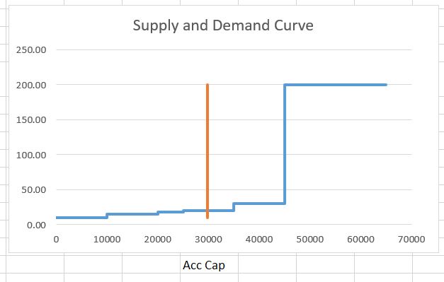
A key idea of this section is that the economics of different strategies depend importantly on the shape of the supply curve. For example, the economics of nuclear power is much higher if the gas price is high. Alternative supply curve shapes are illustrated below. With the steep supply curve, small changes in capacity and in demand and in other factors have a big effect on the marginal and total cost of electricity. In the case with flat supply curves all of these factors have a minor effect.
Creating a Supply Curve – Mechanics
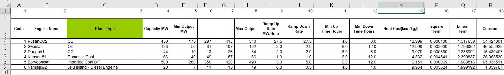
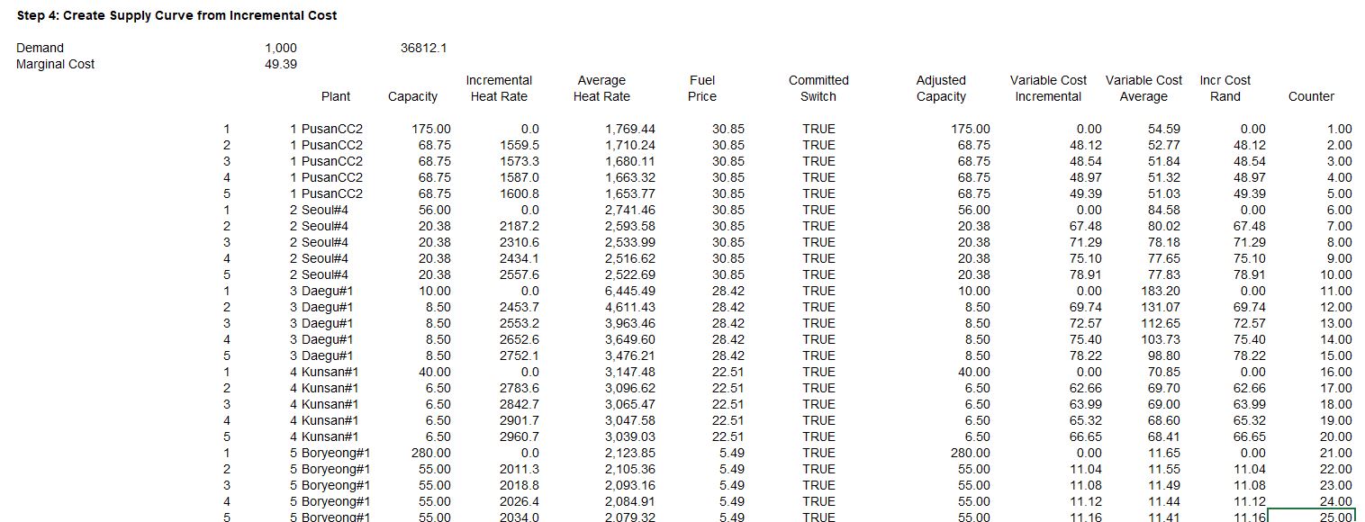
It is a pain to make a nice supply curve for electricity in excel because you should make a step function. To make a supply curve as illustrated below begin with a list of plants and the heat rates etc. and start with a single hour. A supply curve made from a few plants and a level of demand is illustrated on the screenshot below. The file available for download is shown below the screenshot.
- Step 1: Sort the Data by Cost and find a match key
- Step 2: Accumulate the Capacity
- Step 3: Find the marginal unit with the MATCH function
- Step 4: Use the Index Command to Find the Price of the Marginal Unit
- Step 5: Use TRUE and FALSE switch to Find Unit which is Dispatched and Unit on the Margin
- Step 6: Compute the total generation cost using the switches
- Step 7: Construct Counter by 2 to Create Step Graph
- Step 8: Add the Demand to the Graph
Spreadsheet with Simple Short-term Supply and Demand Analysis with Step Function Graph and Demand
The first screenshot below introduces how to make an analysis for a single hour where demand is matched to supply. The manner in which you can create a step function and then combine the supply curve with demand is explained. You begin by entering the plant name, the variable cost of operating the plant (or the bid amount per MWH) and the capacity of the plant on the left. Next you should rank the variable cost of bid from lowest cost to the highest cost. You can add a very small random number to the cost if there are two plants with the same cost. Once the plants are sorted, you can use the match function together with the index function or alternatively the LOOKUP function to find the capacity, the name and other items in a sorted manner. Note that the SMALL function can slow down excel a bit.
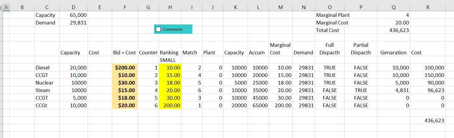
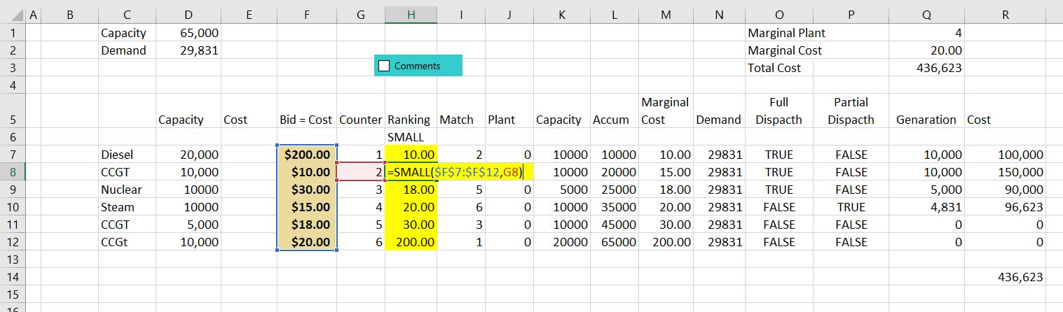
The screenshot below shows how the small function works. This is more effective than using the excel sort function because you may want to add some new plants. In the screenshot, the column to the left of the cost ranking uses the MATCH function where the ranked column is compared to the unsorted bid cost.
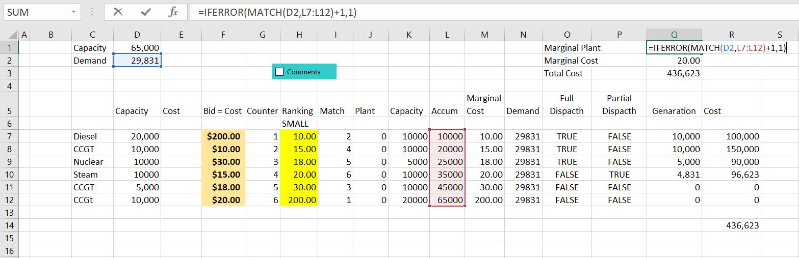
Once the sorted is computed with MATCH and INDEX of LOOKUP (I think LOOKUP is better but this screenshot was taken before I realised this). The capacity is accumulated and then compared to the demand to find the marginal plant. The marginal plant can be found with the MATCH function or the LOOKUP function.
Adjustments for plants with the same cost
- 1. Make an additional column for adjusted costs
- 2. The adjusted costs are the input costs plus a very small random number (RAND() x .000001)
- 3. Use the SMALL command with the adjusted costs rather than the input costs
- Match the demand and the supply
- 1. You can match the input demand with the accumulated capacity to find the marginal price
- 2. You must adjust this because the match command gives the last plant not the next plant
- 3. You must also adjust through reducing the demand by an increment so if the demand matches an increment of supply the marginal cost will be the exact number
- 4. Once you have matched the demand with the supply, use the INDEX command to find the price — the index command is used with the COST
Creating a Step Function Graph
First, to make a graph without a step function can be done with the following steps.
- 1. To graph the supply curve, set up columns as usual with the x-axis (the accumulated capacity) in the first column and the y-axis (the sorted cost) in the second column
- 2. Put a title on the y-axis so that when excel uses the F11 key, it will know what to do.
- 3. Press the F11 key and then modify the chart type to and X/Y chart
- 4. To add the demand to the chart, make a column for the demand that has a constant number
- 5. Modify the chart and use the demand as the x-axis and the sorted cost as the y-axis
If you just graph of the accumulated capacity on the x-axis and the bid price on the y-axis and then make a scatter plot, the graph will look like crap. Tom make a reasonable looking graph using a scatter plot graph, you can follow my method below (maybe there is a simpler way, but this is the method that I use). You have to leave enough rows for two times the number of plants.
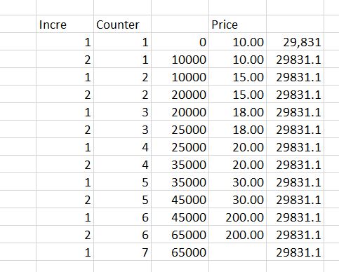
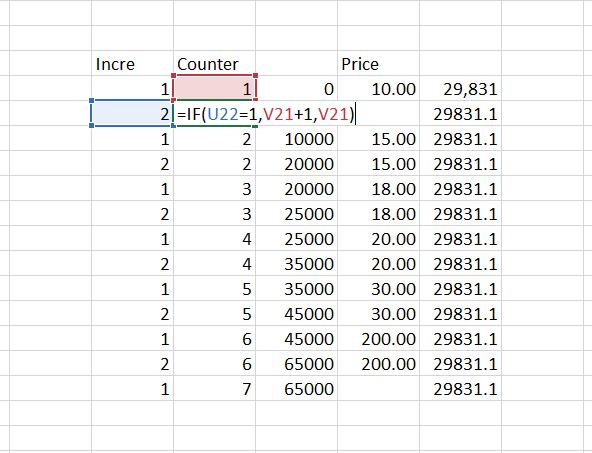
To make a step graph you can start by making an increment that is either 1 or 2. I use and IF statement for this, but there may be a better way. Note how it works — as soon as you hit something other than 1 (i.e 2) then you re-set the number to 1. Note that when you are finished, you will have two numbers for each of the plants. In this way the step will created as there will be two values of the same cost or price for each of the accumulated numbers.
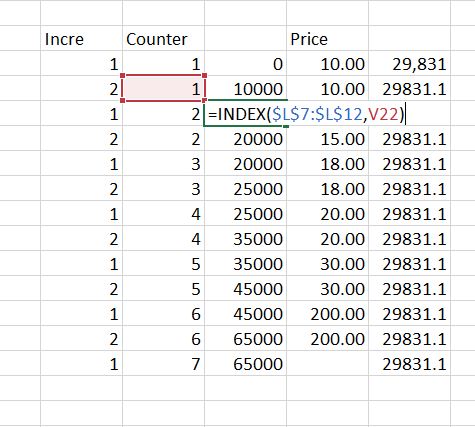
Once the counter is set, you can use the INDEX function in a somewhat unconventional manner. You start with zero and you want the first price to continue for the accumulated amount of the first plant. So you want the x-axis to start with zero and then go to the size of the first plant in MW. Then you want these two numbers to have a value of 10. For the next plant, you want the capacity to begin at the next value and go through the second. To do this, the INDEX function can be used but look to the prior row number.
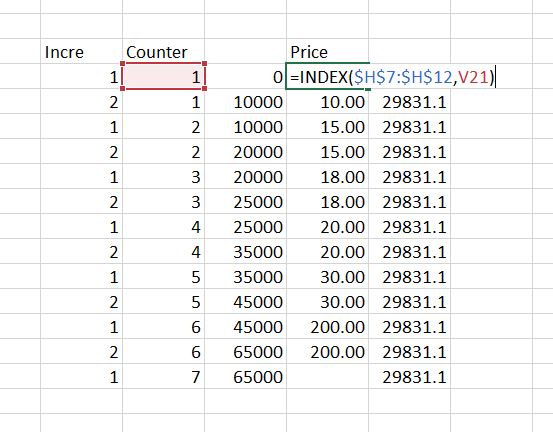
Note in the screenshot below, the INDEX for the price is not staggered. This is how the step function is created with two values of the price for each value. In this case you want two prices with counter. The index is repeated because there are two row values that are the same for each value. Once you have this table made, you can make a scatter plot. To do this, you must make sure the x-axis or the accumulated capacity does not have a title at the top. On the other hand, the y-axis for the price must have a title on the top. Then you can use F11 or ALT, F1 to make a graph. After making the graph, change the chart type to an x-y scatter plot. Then you can make the x-y graph a line graph. Finally, you can put the demand that will be a straight line in the graph.
Incremental Heat Rates and Blocks of Capacity
The file that is attached to the button below demonstrates how the supply curve analysis can be modified to reflect incremental heat rates. The process requires understanding how the average heat rate declines as the plant reaches full capacity. With average heat rates for different blocks, the incremental heat rate is the change in the input MMBTU divided by the change in the output mWh. The three files below contain processes by which you can include incremental heat rate curves in the supply curve.
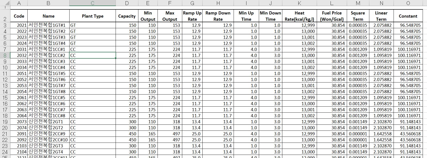
An equation for the average heat rate at different levels of capacity is demonstrated in the two screenshots below. The first screenshot demonstrates how an average heat rate can be represented by an equation with a constant, a slope and a square factor. The second screenshot illustrates the type of characteristics that should be accounted for in a detailed marginal cost analysis.
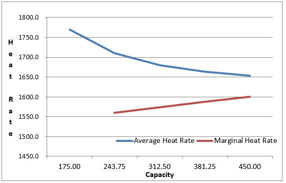
If the plant is dispatched at different levels, the incremental heat rate should change as shown in the screenshot below. To compute the marginal heat rate curve, you can split the plant up and compute the average heat rate that declines. Then, for each block level you can compute the MMBTU input and the MWH output. The incremental heat rate is the change in MMBTU divided by the change in output for different levels of plant operation.
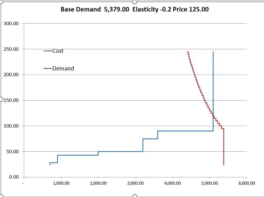
The supply curve with incremental heat rates looks a lot like the supply curve discussed to this point. To model incremental heat rates, you must assume that a plant is on or off. This is why there is a day ahead analysis as well as an hour by hour analysis. The zero cost at the bottom of the graph represents in part the minimum levels of running the plants.
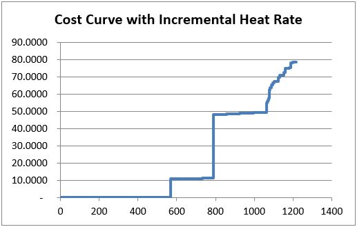
The final screenshot of this section illustrates the supply curve mechanics with the incremental heat rate that is part of the excel files above.
Supply and Demand Analysis in Single Hour that Includes Demand Elasticity to Reflect Demand Response
One of the things that is not done by the supply curve so far is to determine what happens when there is a high level of demand relative to supply. It may be the case that you can reduce demand for a certain price through interruptible rates or demand response mechanisms or with smart meters. The idea of finding more and more load at higher prices is illustrated below.
To perform the calculations of demand elasticity you can use the following equations that are based on the elasticity.
- Elasticity = Ln(Q/Qo)/Ln(P/Po)
- Demand = Base Demand – Elasticity x Qo
- Ln(Demand) = Base Demand – Elasticity x Qo
- Ln(Demand) = Base Demand + Ln(P/P0) * Elasticity * LN(Base)
- Ln(Demand) = Base Demand + Ln(P/P0) * Elasticity * LN(Base)
- Demand = EXP((Ln(P/P0) * Elasticity) * Prior Q
- Elasticity = Ln(Q/Qo)/Ln(P/Po)
- Ln(P/Po) x Elasticity = Ln(Q/Qo)
- EXP (Ln(P/Po) x Elasticity) = Q/Qo
- EXP (Ln(P/Po) x Elasticity) x Qo = Q
The manner in which demand elasticity can be included in the analysis is demonstrated below. Note that there are a number of increments above the total supply.
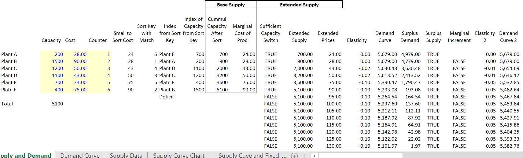
Excel File with Monte Carlo Simulation of Various Items in the Demand and Supply Curve