This web page presents an exercise where you work through the financing section of a project model. In the financing exercise the EBITDA is given along with capital expenditures and various financing assumptions. With these assumptions the assignment that you can follow along is to put all of the equations in the model. The exercise makes you compute the debt size from sculpting and then apply the computed debt size in developing funding source and uses. The exercise includes a flexible method of up-front or pro-rata equity financing, computing IDC which causes a circular reference, creating repayments and debt sizing using sculpting with a given DSCR and programming equations for a DSRA account. I have tried to explain issues in project finance funding using a step by step approach and a video on this webpage. The video explanation where I worked through the file with blank titles and describe various equations. This case uses a copy and paste macro to resolve circular references associated with interest during construction, fees and the DSRA. Please note that the exercise does not include development costs and fees; items that are paid for such as mezzanine ITC that may not be included in the borrowing base; income taxes that cause circular references; use of a letter of credit instead of a cash funded debt service reserve account; sculpting from multiple debt issues; sculpting from P50 or P99; sculpting where the debt size is given by the debt to capital ratio; on-going fees that are included in debt service; VAT facilities and many other items.
It seems that each year I make a new project financing exercise that is relatively simple and that works through debt sizing, debt funding and a cash flow waterfall. Each year I think my last case was not sufficient, well structured, transparent enough, or efficient. So, here is my latest attempt (which may be replaced next year). This time I have started with a time-line, an assumption for EBITDA with fluctuating flows, which because of no working capital changes and taxes, is the same as CFADS. In the video at the end of this section where I work through the answer to the exercise, I explain how I create the time line and I set-up the assumptions. But for the exercise, I begin with a file that includes a titles, the time-line, EBITDA and capital expenditures and assumptions for debt. The file with the input assumptions, the time-line and the EBITDA and Capital Expenditure development is attached to the button below. The idea is that you can download the exercise file and then work through all of the equations by yourself. Then after you have worked through your assumptions you can compare your results with my results (maybe yours are better) and you can watch the video on how I have completed the model.
.
.
.
.
Part 1: Model Set-up and Creating a Time Line in the Exercise File
I have given you the structure of the model by putting the titles in the file. This forces you to follow my structure where I start with a section on debt sizing (this is not a typical part of project finance models, but it often should be). I also believe that a separate section with a summary sources and uses of funds is very effective for setting up the periodic sources and uses of funds and I have included this when I created the titles and the structure. In this exercise, I hope that you will make you equations very simple and very transparent whereby you can find sources with the CNTL [ (followed by F5 and Enter), and you can see the drivers of your equation by pressing the F2 key. I have included a couple of screenshots of the inputs and of the time-line set-up.
Note a few things about how I have set-up the input page. I have put three thin columns to start and then put the category headings in column B (so that column A is the elevator column and immediately goes to the top). The colouring is done with generic macros file — please do not waste time on colouring yourself or using the paint brush. And, please do not think you are a good modeller if you can quickly copy equations to the right. Please download generic macros and be efficient in formatting the sheet https://edbodmer.com/using-generic-macros/
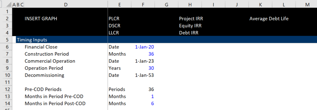
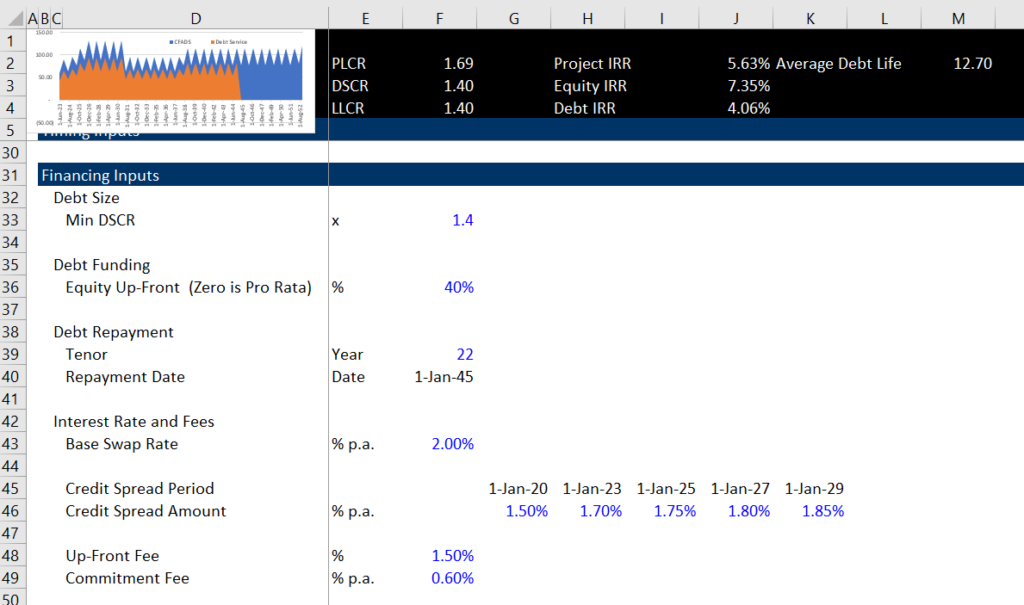
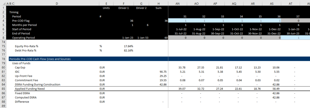
I have started with the financial close and put in a relatively long construction period of 36 months. The screenshot below illustrates the timing assumptions that I have made beginning with the financial close. The screenshot is the top of the input sheet that shows what you are to compute in the exercise including the PLCR, DSCR and LLCR. The DSCR will be the same as the DSCR input because of the assumption that debt is to be sculpted.
.
.
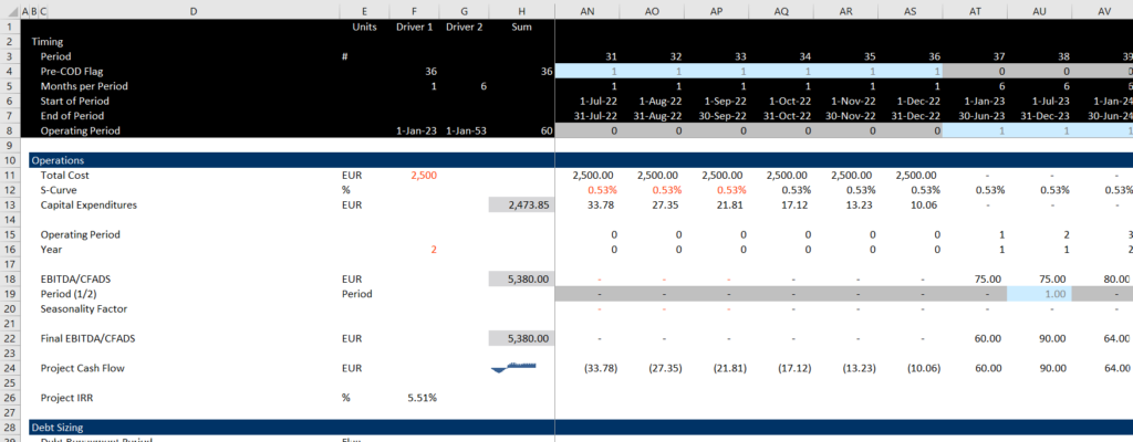
Using these time inputs I have created a master time line on the next page. If you do not have a master time-line that you will eventually use for the IRR and if you have separate time-lines for pre-COD and post-COD your model probably is messed up. The master time line uses the inputs for the number of pre-COD periods and then creates a flexible period from this data in the input sheet. I have made the construction period monthly and the operating period post COD semi-annual to correspond with the assumed debt repayment. The screenshot below illustrates this time-line in the model page along with some of the operating data. Note that I use the columns in the left to guide the model. There is a unit column, two driver columns, sum column and a start column. The screenshot illustrates how the flag for the pre-cod period is created and how the operating period is shown. You will have to create flags as you work through the exercise.
.
.
Part 2 – Review Input for Operations and Financing in Exercise File
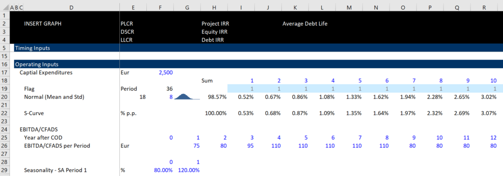
In these exercises I give you the capital expenditures and EBITDA/CFADS already input so you can concentrate on the financing equations. I have put an S-Curve derived from a normal distribution and I have put some varying cash flows and seasonality in the EBITDA. I name the EBITDA/CFADS because the exercise does not include working capital, taxes, LC fees or other items that are between the EBITDA and the CFADS.
The screenshot below illustrates how I have set-up the operating assumptions for the model. I put in some seasonality and changing EBITDA so that you can understand the importance of sculpting for debt size and you can put together a graph of cash flow and debt service.
.
.
When you implement these assumptions in the operating part of the sheet, you can use the LOOKUP or the XLOOKUP function a lot. You should never use VLOOKUP or HLOOKUP or even the MATCH/INDEX combination. In the operation part of the sheet I have created counters for the plant life and the construction period so that you can put the lookup function in seconds. You will have to use the LOOKUP function in the exercise for things like the credit spread that varies over time.
In the courses and in the exercise I do not want you to waste time typing in inputs. So I have given you the inputs. The inputs for debt are arranged to the following categories:
- Debt Size (DSCR or Debt to Capital)
- Debt Funding (Pro-Rata, Equity Up-Front)
- Debt Repayment (Tenure and Type)
- Interest Rates and Fees
- Credit Support
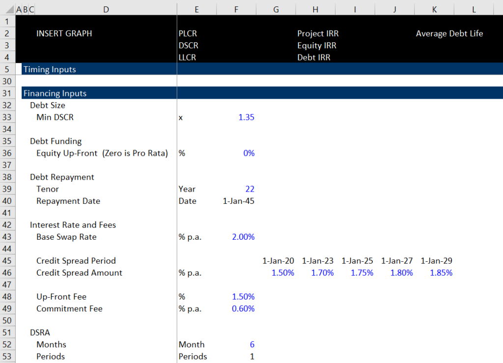
The inputs that I have made for the various debt features are shown in the screenshot below. You will transfer various of these inputs into the driver columns of the model.
.
.
Part 3 – Understand the Financial Structure of the Model with (1) Debt Sizing, (2) Summary Sources and Uses, (3) Periodic Sources and Uses, (4) Debt Balance and (5) Cash Flow Waterfall
After you are finished with the exercise file, your results at the top of the page should look something like the presentation in screenshot below. You can then change the debt parameters and operating parameters and see what happens. For now, please do not worry about the specific inputs as I have changed some of the inputs for the target DSCR, the debt tenure and other variables. I just want to show you the key outputs that you will be ultimately deriving when you have completed the exercise. I argue that the essential graph in a project finance model is the graph with cash flow and debt service illustrated at the top left of the the screenshot.
.
.
Before working on the case, you should understand how I have set up the model structure. Please be creative and do not follow blah blah rules. I have put in a section for debt sizing which is the first part of the exercise that you should work on. This is generally not a separate part of models. Then I have put in a summary sources and uses of funds that I consider essential. After that, you can much more easily fill in the month by month funding section with the MIN function. Finally, the model is finished with the debt accounts that are always part of the model along with a post-COD cash flow waterfall. I emphasize that you should not be wedded to a particular structure and you should be flexible and creative in your modelling. In this case with the debt size determined by sculpting I believe the model should start with operations and not development, construction, construction financing, operations, debt repayment and financial statements that is in many other models. I have included a video that describes the set-up of the model, the time line and how to create the exercise below.
.
Part 4 – Completing the Debt Sizing Section
The first section for you to complete in the exercise file is the debt sizing section. This section applies fundamental mathematical rules that:
NPV of Debt Service is Debt at COD
and that NPV can be computed using the SUMPRODUCT with the Debt Service divided by and index of periodic interest rates that begins at 1.0 at the date of the COD. Yes, you can divide in the SUMPRODUCT.
NPV = SUMPRODUCT(Cash Flow / Compound Discount Factor)
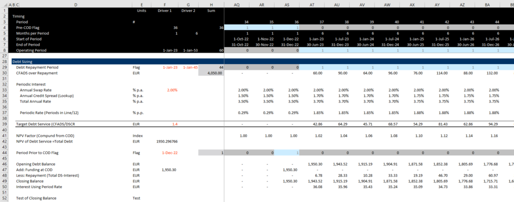
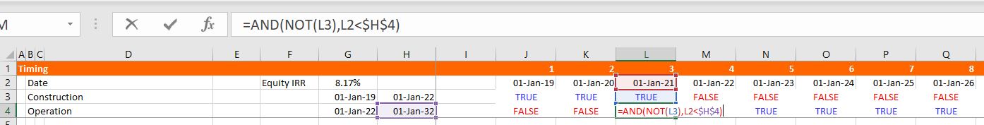
The screenshot below illustrates the process. First compute a debt repayment flag with the AND function using the starting date compared to the COD and the debt maturity finish. Then multiply the CFADS by the debt repayment flag. Get the interest rate from the input sheet using the LOOKUP function and then compute the periodic interest rate as the annual interest rate/12 * months in period at the top of the page.
Use the periodic interest rate to compute an index that begins with 1.0 at the COD date — you can use the formula:
Index = prior * (1 + periodic rate * operating flag)
With the index you can compute the debt size as:
Debt size = SUMPRODUCT(Debt Service/Interest Factor)
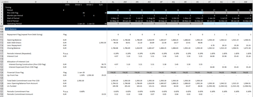
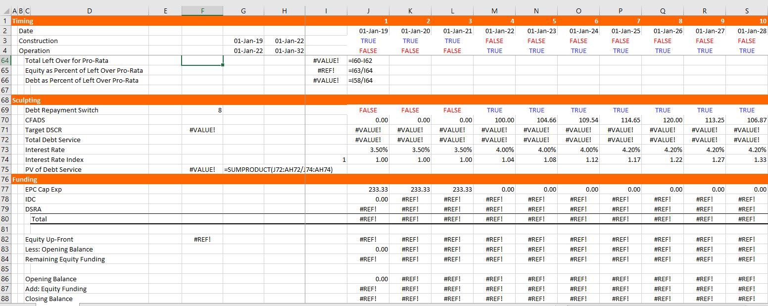
To complete the debt sizing, you can compute the debt balance using a flag that is one month before the COD date and then use this flag for the draws. The repayment is just debt service minus interest and interest is computed from the opening balance multiplied by the periodic rate. These equations are illustrated in the screenshot below. Note the debt sizing title, followed by the CFADS over the repayment period.
.
.
.
Part 5: Summary Sources and Uses Section
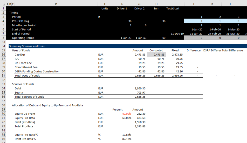
Once you have completed the debt size, the next section of the model for you to complete is the summary sources and uses section. This is generally not included in models but I strongly believe it should be. With the summary uses and sources you can show you copy and paste circular references in a transparent manner and you can use the balances to compute items in the construction funding part of the model (that I call the monthly uses and sources). I have put in titles for the capital expenditures and IDC and Fees and DSRA as shown below. Note that you can find the capital expenditures from the sum above, but you will have to put in the IDC, fees and DSRA later on and it will create a circular reference. After you put in the capital expenditure sum and a place holder for the sum of all of the uses, you can put in the debt from the debt sizing section. Finally, the equity is just the total uses minus the debt.
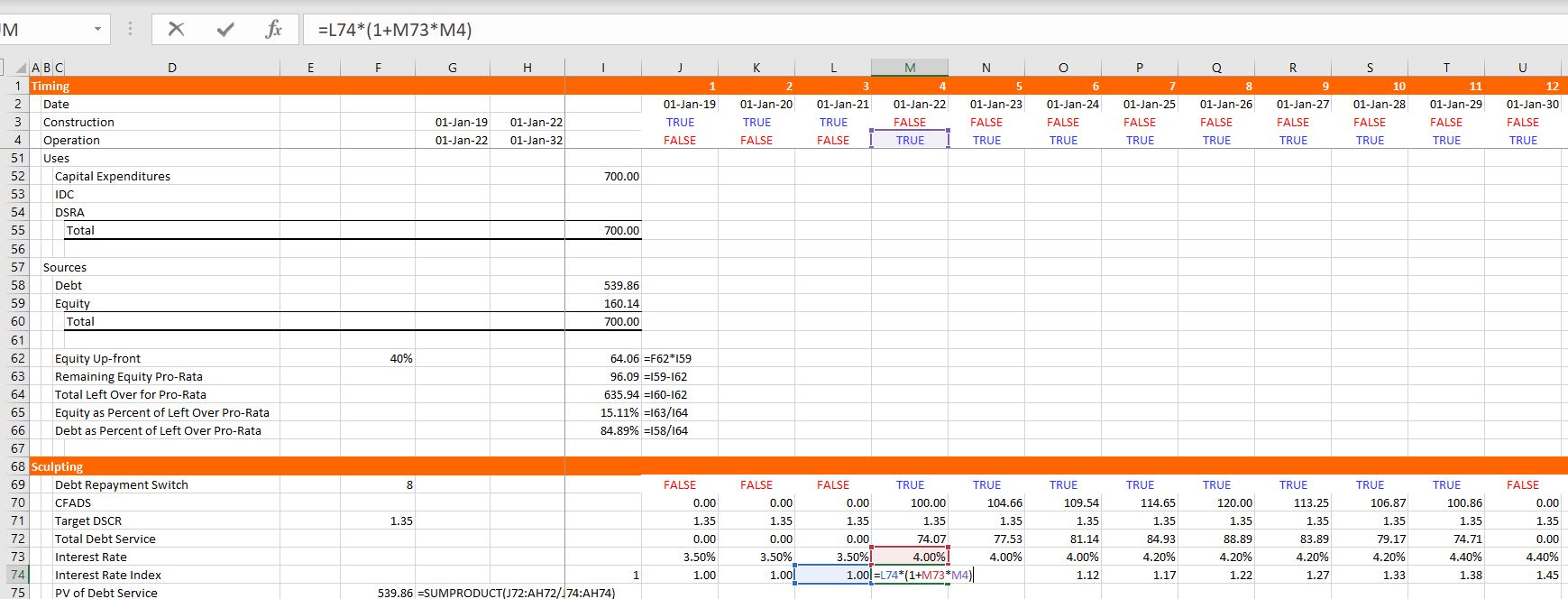
The screenshot below illustrates this. At the bottom of the sources and uses I show the amount of equity allocation to up-front equity and to pro-rata equity. (You may often have to divide up the equity into different parts such as EBL or shareholder loans). The pro-rata percentages are the final part of this section below the sources and uses. The pro-rata can be computed by adding the debt and the equity pro-rata and then computing the percentages.
.
.
Part 6 – Periodic Cash Flow Pre-COD – Monthly Uses and Sources or Construction Financing
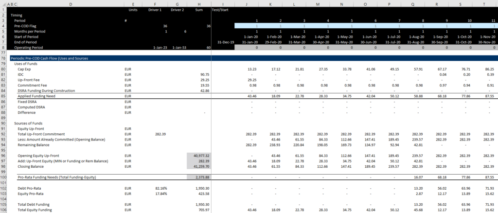
In the next section, you can compute the funding requirements with the same titles as the summary uses of funds. Except, rather than putting in the sum, you put in the period by period capital expenditures. Again, you are not ready to put in the period by period IDC, fees and DSRA because these have not been computed yet. As with the summary sources and uses, compute the sum even though all the components (IDC, fees, DSRA) are not there yet.
Once you have the funding needs, the task is to allocate the funding needs to debt and equity. The equity funding is split between up-front equity and pro-rata equity. You can compute the total equity commitment and subtract the opening balance of a separate account for the up-front equity. This will provide the remaining balance:
Remaining balance to Fund = Up Front Commitment – Opening Balance
The amount of equity funding is then computed as the minimum of the funding needs and the remaining balance:
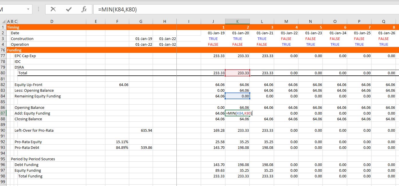
Equity Funded Up Front = MIN(Remaining, Funding Needs)
After the up-front equity is computed, you can compute the pro-rata funding of debt and equity. This is precisely why I computed the pro-rata percentages in the last section (look at the bottom of the screenshot above). So, you first compute the total pro-rate funding as the total funding needs less the up-front equity funded. Then, you split the pro-rata funding into debt and equity according to the percentages.
.
.
Part 7 – Debt Balances with Interest Allocation and Fees
In the next section you can compute the balance of the debt issues with the opening balance, draws and repayments. You can get the repayments from the debt sizing section and the draws from the funding section that was just discussed. You can then get the interest rate from the debt sizing section were we computed the periodic interest rate. Put an opening and closing balance together, get the draws and repayments and then compute the total periodic interest cost (monthly and later semi-annual). Then you can collect the total debt from the sources and uses statement to compute the up-front fees and the commitment fees. These two calculations depend on the debt commitment directly.
The screenshot below illustrates how you can complete the debt balance calculation from the summary uses and sources as well as the construction financing. Finally, the amounts of IDC and fees can then be put back into the periodic construction financing sources and uses. But once you put the sum of the values into the summary sources and uses you will get a circular reference.
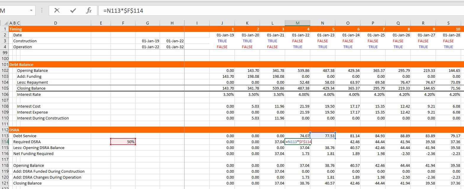
Part 8 – DSRA Section
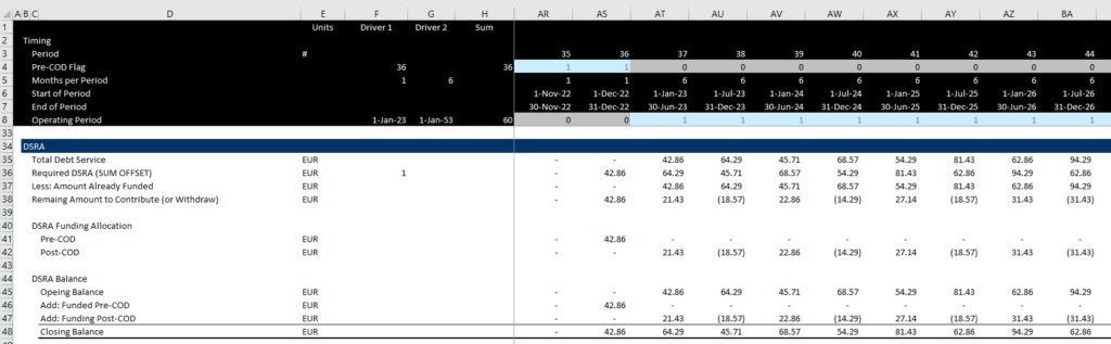
Modelling the DSRA can be painful. But to get started, first compute the required DSRA. Then you can compare the required DSRA with the amount that is already funded. The difference between the required DSRA and the amount that is funded is the amount that must be contributed to the DSRA account and the amount that can be withdrawn from the DSRA account. This is shown at the top of the screenshot below. The trick for this is to get the amount already funded from the opening balance of the DSRA account. Once you have computed the amount to contribute or withdraw, you can allocate the amounts to the pre-COD period or the post-COD period with the flags at the top of the sheet. You should make this allocation because the pre-COD goes into the sources and uses construction financing and the post-COD goes into the post-COD cash waterfall. There is a painful equation for the amount of the required debt service once you have the debt service. You should look forward one period and then accumulate the number of periods to sum. To do this you can use the formula below:
Required Debt Service = SUM(OFFSET(Debt Service,0,1,1,Periods to Sum)
.
.
Part 9 – Circular References from IDC, Fees and DSRA
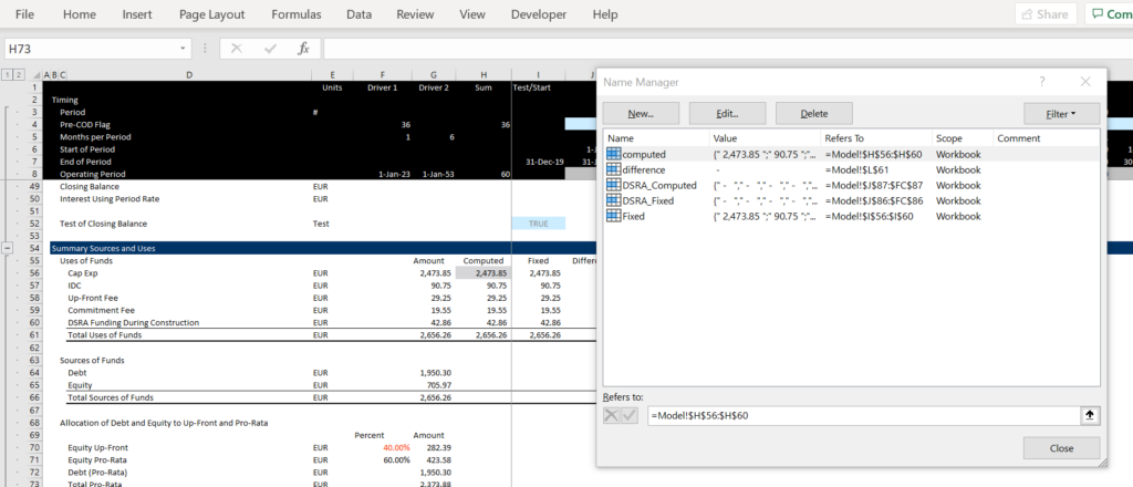
Once you have finished the DSRA, you go back up to the monthly sources and uses of funds and then fill in the monthly IDC, the monthly up-front fee, and the monthly commitment fee. When you first fill in the numbers you will not see the dreaded blue lines for circular references. This is not the case when you link the pre-COD contributions to the DSRA. So wait with the DSRA for a minute. After linking the monthly values for IDC and fees, compute the sums in the left column as you would do for any account. This should still be ok. But when you put the sums up to the summary sources and uses you should get a circular reference. First, make a range name around columns for the fixed and computed ranges for IDC, fees and DSRA. The range names are illustrated on the screenshot below.
.
.
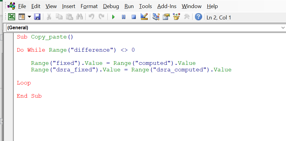
With the range names, you can then create a range for the difference between computed and fixed. This is in the difference column of the summary sources and uses of funds after you make the column for the fixed and computed values. Assign the applied column on the left for the summary to the fixed value can create a macro to copy to the fixed from the computed. Then compute the total difference column. Put the range name for the difference into the the macro with a Do While as shown below. To copy from the computed to fixed you can use RANGE(“range_name”).value as shown below.
.
.
You can attach this to a button and then run the copy and paste macro and start working on the DSRA circular reference which is more difficult. The DSRA requires you to compute fixed and computed values for the entire line. The first thing to to is to insert lines for fixed and computed DSRA values as illustrated in the screenshot below. Then make range names around the entire rows. The computed value comes from the pre-cod value that was discussed in the last section. Then the applied number comes from the fixed value. As with the summary, you should compute the sums and this time compute the sum of the difference. Once you have done this put the range for the computed and the fixed values in the macro as shown above. If this is too confusing, you can watch the video below that goes though the entire solution.
.
Part 10 – Cash Flow Waterfall Post-COD and Outputs
With the circular reference resolved you can now compute the cash flow waterfall. In our example, this is very simple. The main thing you do in our simple case is to link up to the EBTIDA, link the interest and repayment and link the DSRA withdrawal amounts that provide positive cash flow. The final number in the cash flow waterfall is the dividends. With the dividends and the cash contributions from the periodic cash flow you can compute the equity cash flow and the equity IRR. To compute the equity IRR use the XIRR formula with the ending dates to be consistent with the interest assumptions that use opening balance and presume that the cash flows occur at the end of the period. After computing the equity IRR you can compute the DSCR from the cash flow statement. You can use an if statement and then not put in anything for the false:
DSCR = IF(Debt Service > .1, CFADS/DS)
This gives you a FALSE when there is no debt service. False is much better than 0 because than you can compute the minimum and average etc. The DSCR better be the amount that you entered in each period. It compute the LLCR calculate the CFADS over the debt period and then use the SUMPRODUCT with the interest rate index you computed in the debt sizing section to compute the PV of CFADS. Divided the PV of CFADS by the debt balance to compute the LLCR. The PLCR is the same calculation but you use the CFADS over the entire life of the project. To compute the debt life create a counter for the debt period. Multiply that counter by the debt repayment, sum the product and divided it by the total debt at COD. Compute the debt IRR from all of the debt cash flows, positive for fees and debt service; and negative for the debt draws. Finally, you can make the graph using the NA() trick. The NA() trick is discussed in detail at https://edbodmer.com/na-trick-and-flexible-x-scale/
Part 11 – Final Completed Case
The button below is attached to the completed case. This case is described in the video.
.
.
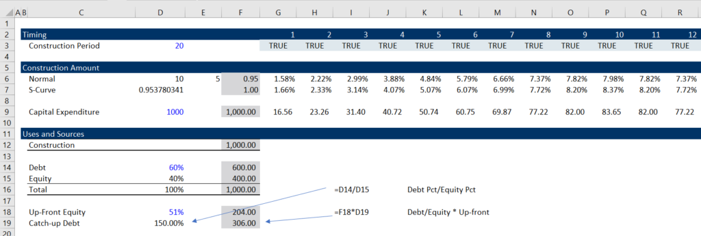
Other Issue — Pro-Rata, Equity Up-Front and Catch-up Debt
In the above example, I assumed that if there was some up-front equity and some pro-rata, then the up-front equity would be issued and after that, all of the financing would be pro-rata. An alternative assumption could be that after the up-front equity, there is a period of all debt. I call this catch up debt. After the catch-up debt, the financing reverts to pro-rata at the debt to capital and equity capital at the input ratios. To model this, I suggest you create a simple case without other junk to isolate on the issue. The first thing to do is to set-up the summary sources and uses as usual. Note that you first compute the debt divided by equity in column D. Then you multiply this percentage by the up-front equity.
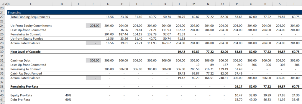
Next, you can make a real cash flow cascade. You start with the total financing requirements. Then, as usual, you compute the up-front equity. This leaves some funding for the catch-up debt. You can then make the same calculation with the total catch-up commitment, the remaining commitment and the opening and closing balance of the catch-up debt. Once the commitment is filled and the remaining balance goes down to zero using the MIN function, you can compute another level of the cascade. This remaining amount can be computed using pro-rata ratios.
.
.
Sculpting playlist.
.
.
.
.
.
.
.
.
.
.
.
.
Legacy Exercise 2 from 2019, Part 1 — Overview of Exercise, Colouring and Interpolate
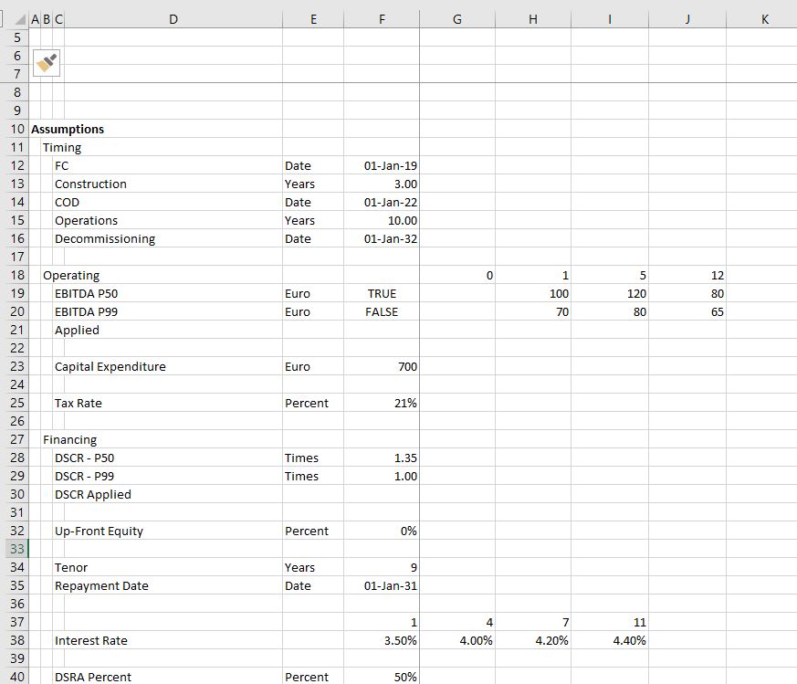
After you open the file, I suggest that you look over the inputs and the structure that is defined by the input titles. The given inputs are shown in the screenshot below. You can first open the generic macros file (link provided) and format the colours of the inputs as well as the different sections (press CNTL, ALT, C). This will make make some nice colours — please do not waste time colouring and formatting. I used an annual time line (not the typical case where you would put the construction in months) to save a bit of time. The EBITDA input has an option for P50 or P90 so we can later compute the tariff from the P50, while the debt sizing may come from either the P50 or the P90. The inputs include funding options with different up-front percentages; it has debt sizing from the DSCR and sculpting; it has changing interest rates and it has a funded DSRA.
[wonderplugin_video iframe=”https://www.youtube.com/watch?v=S6axzpDxyVQ” videowidth=600 videoheight=400 keepaspectratio=1 videocss=”position:relative;display:block;background-color:#000;overflow:hidden;max-width:100%;margin:0 auto;” playbutton=”https://edbodmer.com/wp-content/plugins/wonderplugin-video-embed/engine/playvideo-64-64-0.png”]
Legacy Exercise 2: Part 2 – Enter Time Line Switches and Dates
After looking at the layout, put in the dates at the top of the file. Use the EIS (in french you can find the series in the main menu and find the short-cut with the series you can go to the short cut page by clicking on this link. In English (ALT, H, FI, S). Enter the dates as illustrated in the formula the little screenshot below. I used EDATE (in french this is something like DATE.MOIS). If you have the generic macro file open, you can then use SHIFT, CNTL, R to copy the dates to the right. Note that the screenshot has nicer colours because of using CNTL, ALT, C in with the Generic Macro file open. Once you have the dates you should enter the switches (you can call these masks or flags and you can use 1,0 or TRUE, FALSE). Use the SHIFT, CNTL, R to copy to the right. To summarise, put the numbers of the period at the top. Then link the very first date to the financial close. In the cell to the right, use the EDATE function and press SHIFT, CNTL, R. Below the dates put a construction and operation switch. You can put the start and end dates to the left to document what you are doing. For the construction period, the dates at the left are the financial close date and the commercial operation date. For the operation period, use the commercial operation in the left most column and use the decommissioning data in column H. Once you have the dates, use the AND function (E in french). You always refer to the date line in row 2. For example, for the construction switch use the formula AND(date>= FC date,date<COD). For the operation flag or switch, the formula is AND(date>=COD,date<DECOM).
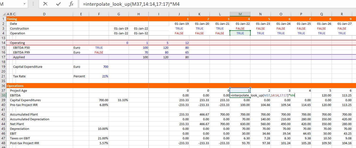
One thing that may be a little tricky in the model is to compute the EBITDA from either the P50 or the P90. The calculations of EBITDA are displayed in the screenshot below. You can use the TRUE and FALSE inputs in column H to chose which scenario is in place (the false in cell H16 is NOT(H15)). In the screenshot below, the numbers in line 17 are computed with the TRUE and FALSE. To implement either the P50 or the P90, you go to line 17 and multiply the numbers in the P50 line (line 15) by the TRUE or FALSE in column H and you do the same with line 16 for the P90. The formula for line 17 is: TRUE * Line 15 + FALSE * Line 16, where the TRUE or FALSE come from the items in column H. Then, the idea is to interpolate the EBITDA rather than using a step function that you can compute with LOOKUP (RECHERCH in french). You can see how the LOOKUP function works by going to the associated link. Then you can try to interpolate the EBITDA numbers instead of using the LOOKUP function. To do this you should try to use the INTERPOLATE LOOKUP function that I created and that you have to bring into your file (the link is provided to retrieve this function with instructions on how to upload the function). The manner in which you can compute the EBITDA from a counter and the INTERPOLATE function is shown in the screenshot below. You should make the counter by accumulating the operating switch. Then you should use the entire row with the LOOKUP or INTERPOLATE LOOKUP function. (If you are having trouble bringing in the INTERPOLATE function, use the LOOKUP function and model EBITDA as a step function). The LOOKUP function starts with one input that corresponds to the item that is being looked up — it is typically a date or a counter. To implement LOOKUP or INTERPOLATE, you then put in the entire row for the corresponding item — in the case below, this is line 14. Then you click on the entire line 17 that will arrange the EBITDA. Finally you should multiply the INTERPOLATE formula by the TRUE or FALSE for the operating switch as is shown on the screenshot. Use the SHIFT, CNTL, R to copy to the right. (Notice how there is a freeze pane for the dates and the switches). I think it is worth giving up completely on VLOOKUP or HLOOKUP (in french RECHERCHV or RECHERCHH). After you have created the EBITDA, the rest of this portion of the model to compute the pre-tax project IRR and the post-tax IRR (TRI in french). Pre-tax IRR is computed from pre-tax cash flow which is EBITDA less Capital Expenditure. Then compute depreciation expense and use the depreciation expense to compute EBIT. With the EBIT you can compute the operating taxes and the after-tax cash flow.
Legacy Exercise Part 3: EBITDA and Project IRR
Part 4: Summary Sources and Uses and Debt Size from Sculpting
The next step of the model is to set-up a summary sources and uses of funds statement and a sculpting schedule to evaluate the the debt size. In this case, assume that the size of the debt is driven by the minimum DSCR and the minimum DSCR is applied for each period. You can fill in the sources and uses except for debt items which is very simple — just sum up the capital expenditures and compute the equity as the total cost less the debt. To find the debt size from sculpting, you can go to the sculpting section just below the sources and uses as shown in the screenshot below. For now, fill in the CFADS line with the EBITDA instead of CFADS (which is of course not correct). Use the SHIFT, CNTL, R to copy to the right. You should also multiply the CFADS by a debt switch that contains a TRUE in the periods of the debt repayment. Then compute the debt service as the CFADS divided by the DSCR and apply the SUMPRODUCT with and interest rate index in computing the NPV of debt service which is the the size of the debt. If you want some more background on basic sculpting, go to the associated link. Note that you should make sure that the DSCR is working with the TRUE and FALSE for the P90 or the P50 DSCR in the assumptions section. Once you put the debt amount from the PV of the debt service into the sources and uses, you can work on the pro-rata percentages used for computing period by period funding. Pro-rata percentages compute a pro-rata base that is the non-up-front equity plus the debt (note that all of these numbers must be reduced by the capitalised interest). I hope you see how useful it is to have a summary sources and uses of funds.
Part 5: Funding During Construction Cash Flow Statement
A project finance model has two cash flow statements. You probably know the cash flow waterfall after construction that occurs after the COD. The other cash flow is the cash flow statement before the COD that works through how much funding is required and where the money comes from. The screenshot below illustrates the funding section. Begin with the same titles that are in the uses of funds including the EPC cost, the IDC and so forth. Fill in the items on a period by period basis. Then begin with the up-front equity. To model how much up-front equity can be used I suggest setting up a little table that evaluates how much remaining up-front equity must be used before pro-rata funding kicks-in. Once you have this table you can compute the up-front equity funding using the MIN function as shown in the screenshot below. The MIN function is MIN(Funding Needs, Remaining Funding). After the up-front funding, you can enter the pro-rata percentages to the left and then compute the funding from equity and debt pro-rata funding. These percentages which are shown in the screenshot below come from the summary sources and uses analysis.
Part 6: Debt Schedule and DSRA Schedule
With the funding defined and the sculpting defined, you are ready for the debt schedule which keeps track of debt balances and derives interest expenses. To keep things less tedious, fees are not included in this example which is illustrated in the screenshot below. Once the debt schedule is complete, you can use the debt service to compute the required DSRA balance and the DSRA account. The debt schedule is pretty standard with the opening and closing balance, repayment and interest. In order to compute the repayment, just use the idea the debt service is equal to interest plus repayment which means repayment is debt service minus interest. Then you can go to the debt service line and subtract the interest from the bottom of the debt balance. With the debt balance you can compute the DSRA. You can take the pain out of computing the DSRA by starting with the required DSRA at the top of the section. This required DSRA is the debt service from the debt schedule in the subsequent year multiplied by the DSRA percent. Then, when you have the required DSRA, you can subtract the amount already in the DSRA (the opening balance of the account). Once you have the required amount of the DSRA, put in an opening can closing balance and add the required funding. But when you add the required funding (which will eventually be negative), you should split it between funding during construction and funding during operation (which will eventually be negative). To do this, multiply the required funding by the operating switch or the construction switch.
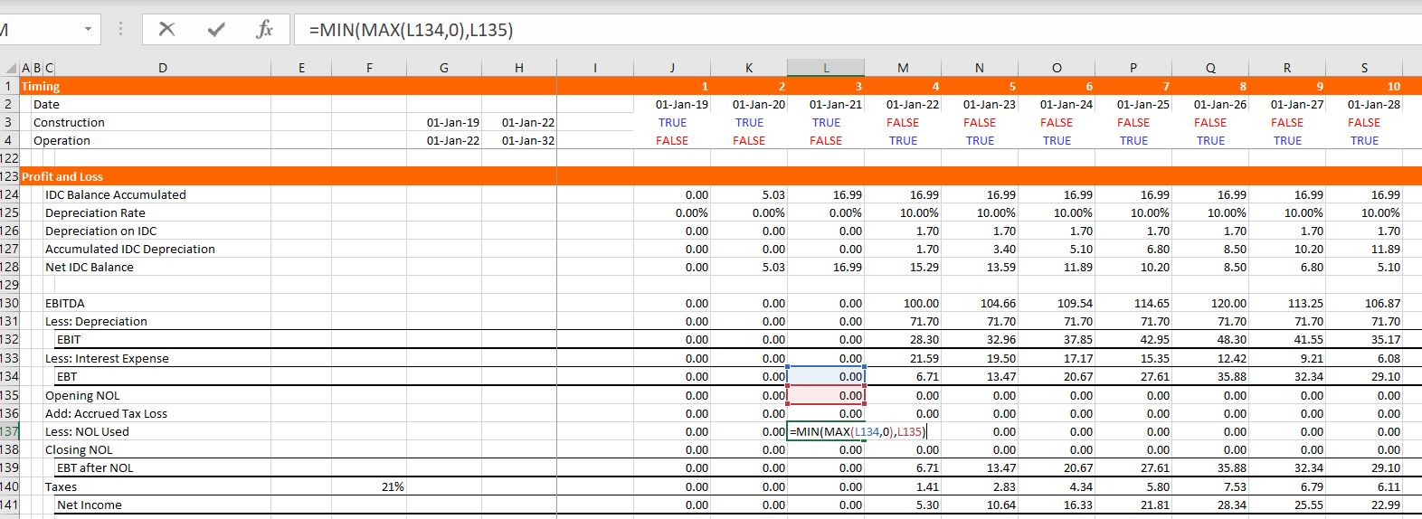
Part 7: IDC Depreciation and Profit and Loss
CFADS is computed as EBITDA less taxes which means that you need to compute taxes and, in turn, you need to work through a profit and loss statement. You already have EBITDA, interest, and a tax rate from other items in the model, but the depreciation expense must be adjusted for IDC. So, in the screenshot below, you can see that I put IDC depreciation at the top of the P&L. This is not very conventional, but I do this to illustrate the flow of the model and the fact that IDC deprecation cannot be computed until after the debt schedule is computed. To compute IDC depreciation, accumulate the IDC, use the depreciation rate from the basic deprecation calculation above and compute the accumulated depreciation. Next, you can work through the income statement and get to the tax page. In computing taxes, there may be a net operating loss. The NOL can be computed by setting up a balance account and increasing the NOL when the EBT is negative. This can be accomplished by using MAX(-EBT,0). The NOL is used when the EBT is positive and the opening NOL balance is positive. This can be modelled using MIN(MAX(EBT,0),Opening Balance) as shown in the screenshot. Once you have the additions to the NOL and subtractions from the NOL, you can compute an adjusted EBT calculation and the taxes paid. The adjusted EBT is the EBT before the NOL plus the addition to the NOL, minus the use of the NOL.
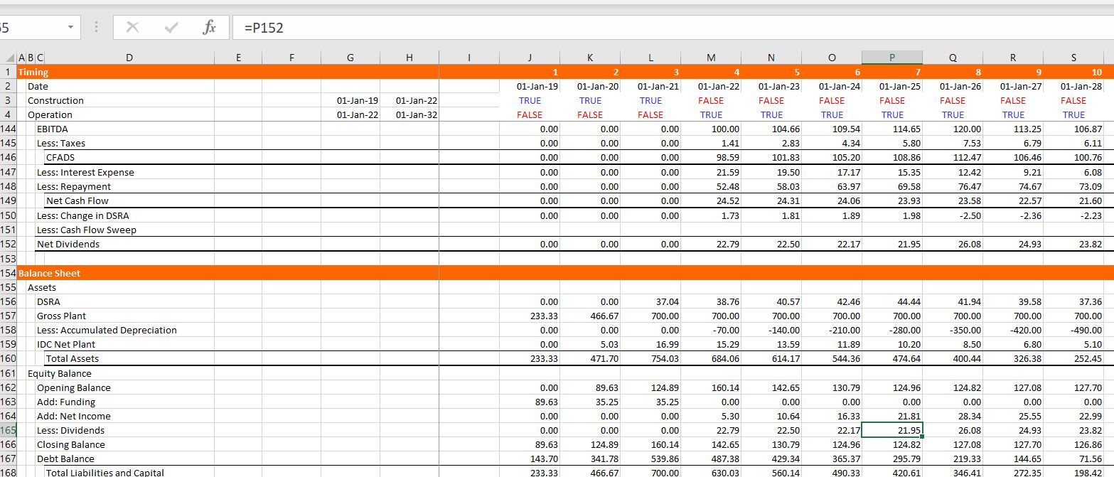
Part 8: Cash Flow Waterfall and Balance Sheet
We are finally just about finished with the model, we just need the cash flow statement and the balance sheet. With one exception, these two statements involve just finding other rows, linking the formulas and then computing a few sub-totals as shown in the screenshot below. For the cash flow statement, just start by linking the EBITDA, the taxes, the interest expense, and the repayments. In constructing the balance sheet, just go up and find the closing balances of various accounts like the plant balance, the accumulated depreciation, the debt and the IDC plant balance. The exception is computation of common equity. For common equity set-up an account with the opening and closing balance. Add the funding which is the last line of the funding cash flow statement; add the income which is the last line of the profit and loss statement; and, subtract the dividends which is the last line of the cash flow waterfall as shown in the screenshot. When you do this, the balance sheet does not balance. This is because the IDC from the debt balance has not been attached to the funding statement and the DSRA funding has not been attached and the sum of the IDC funding requirements and the DSRA funding requirements are not in the summary sources and uses statement.
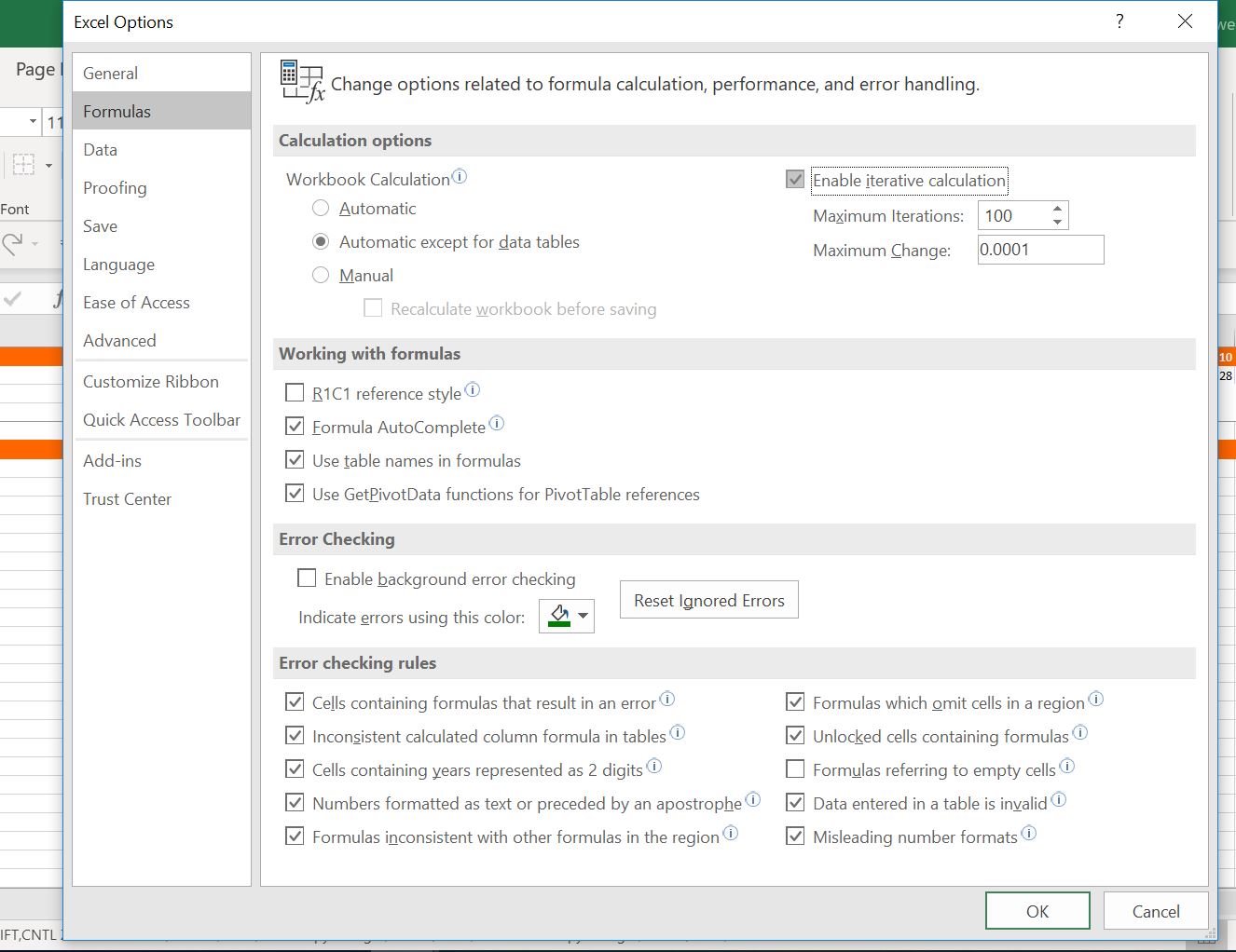
Part 9: Circular References and Iteration
It is really painful for me to suggest this, but to finish this part of the model can you use the iteration button in excel. The screenshot below shows you how to do this, but I really hope you will hardly ever use it. I explain elsewhere that when you put in a bad input; when you make a mistake; when you try to use the goal seek, your model blows up. But let’s go anyway and then see what happens when you make these errors. First go to the IDC line in the funding section and fill in the amount from the interest during construction in the debt. Then stay in the funding section and go to the DSRA. You can attach this line to the line with the DSRA funding during construction. Next, continue going backwards and put the sum of the IDC from the funding section into the sources and uses summary. Do the same for the sum of the DSRA function, namely put the sum of the DSRA line in the funding section into the summary sources and uses. Finally, go to the sculpting section and replace the EBITDA that we used with the CFADS line way down in the cash flow statement. Once you do this, the balance sheet should balance. Finally compute the DSCR and the equity IRR. The sDSCR should be the same as the target. To compute the equity cash flow, you can look up in the balance sheet and find the equity funding and the dividends. The dividends are positive cash and the equity funding is negative.
In this final section I will show you a couple of problems with using the iteration button. First you must save the file. Next make an error in the input. Put the letter a in the DSCR. You will get a bunch of errors in the model. Then press CNTL Z to undo. This does not clear the errors. Now delete the debt service row in the sculpting section (after re-opening the model) – use CNTL – and remove the row. This time you will get a bunch of #REF’s. Try to undo again and it still does not work. So, you better close the file and re-open it again. Now try to use the goal seek. Why don’t you set the IRR to 10% by changing the last EBITDA. The goal seek just goes around and around and does not work.
The button below has the completed file. You can check your work or just look through the file.
Playlist on Sculpting Issues
If you are in the mood for torture or maybe if you are having trouble sleeping, you can look through the sculpting playlist. I have put together various sculpting videos that I have made over the years. I have tried to put the more basic videos first (with the exception of the very first). The videos all apply the fundamental formula that the PV of debt service over the repayment period is equal to the debt size at the beginning of the repayment period (i.e. the period just prior to the commercial operation date). Over time I have learnt more about sculpting issues that can involve curved DSCR’s, multiple debt issues, incorporation of on-going fees, alternative debt sizing options, complex income taxes and computation of DSRA moves as part of the CFADS. I hope I have covered a lot of these issues in the videos. As with other items, you can always send me an email at edwardbodmer@gmail.com.
.
.