Automatic Read with Interactive Data
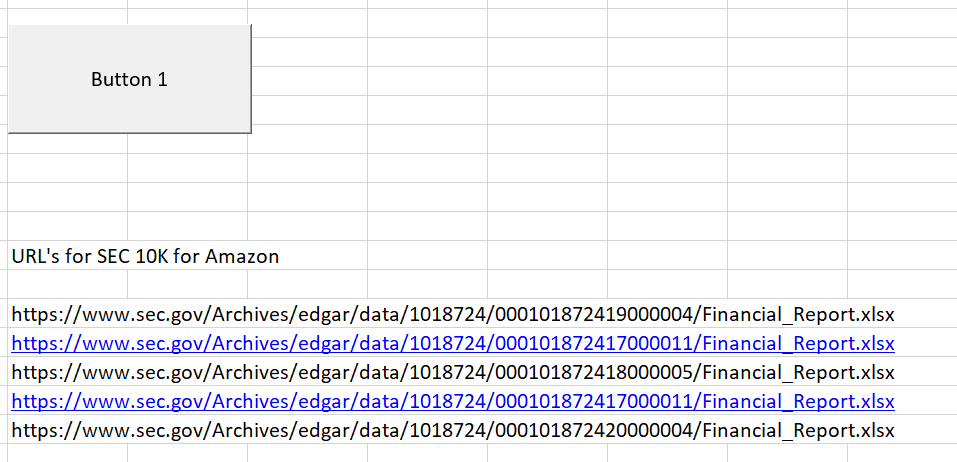
Since 2009, you can download financial statement data directly into an excel sheet. This is fantastic except that it is clumsy to manually download data, then put the data together from different years and then re-formatting the data. I will work through how to create VBA code to make the process work much more quickly. The first step to making the process more automatic is to create a macro that reads the data and puts the files into a defined folder. To see how this works, go to a page like this and right click on the red text that says “View Excel Document”. When you right on the text named to “View Excel Document” which will find the appropriate URL. After that copy the address and you will see a URL like the one below. The link below is for Amazon with a code of 1018724.
It is easy to put this link into workbooks open. But the number at the end is not the same. So instead you can use an error checking routine. Different URLS’s for Amazon for different years are shown in the screenshot below. Note that the final numbers are not all the same.
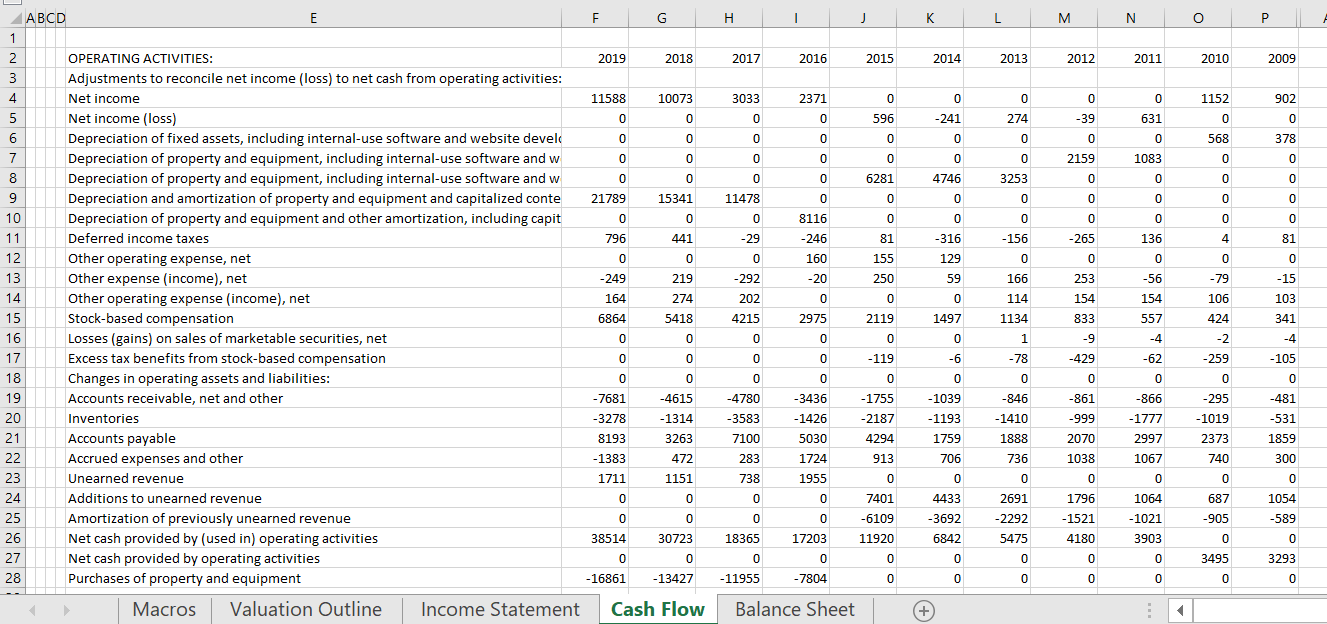
Once you read in the URL’s, you can put the files together into different sheets. I have created a macro that works through data once you have the company code number used by the SEC. The screenshot below illustrates how you can filter through different files published by the SEC and save the files. The files are saved into an area you define. Once you have the excel files defined, you can put the income statement, the cash flow statement and the balance sheet together. I have made macros with short cuts (SHIFT, CNTL, I) for the income statement (SHIFT, CNTL, C) for the cash flow statement and (SHIFT, CNTL, B) for the balance sheet. This allows you to quickly open the financial statement files and then put them together.
Using the Union Function to Put Together Financial Statements
I have tried to make a very painful process as easy as possible. I have not been able to make it fully automatic, but I hope you can get a file together if minutes rather than days. Like many functions, the UNION function is an array function. This means the output does not go into one cell but rather into a series of cells. To operate the UNION function you should leave a long space and then select the long space. After that, you begin typing the UNION function. Then like with any function press the tab key. After that, you can select multiple other columns (or rows) that will be combined into one single column, At the end press the SHIFT, CNTL, ENTER sequence.
Here is a step by step review of the union function:
Step 1: Insert some columns at the left of the sheet
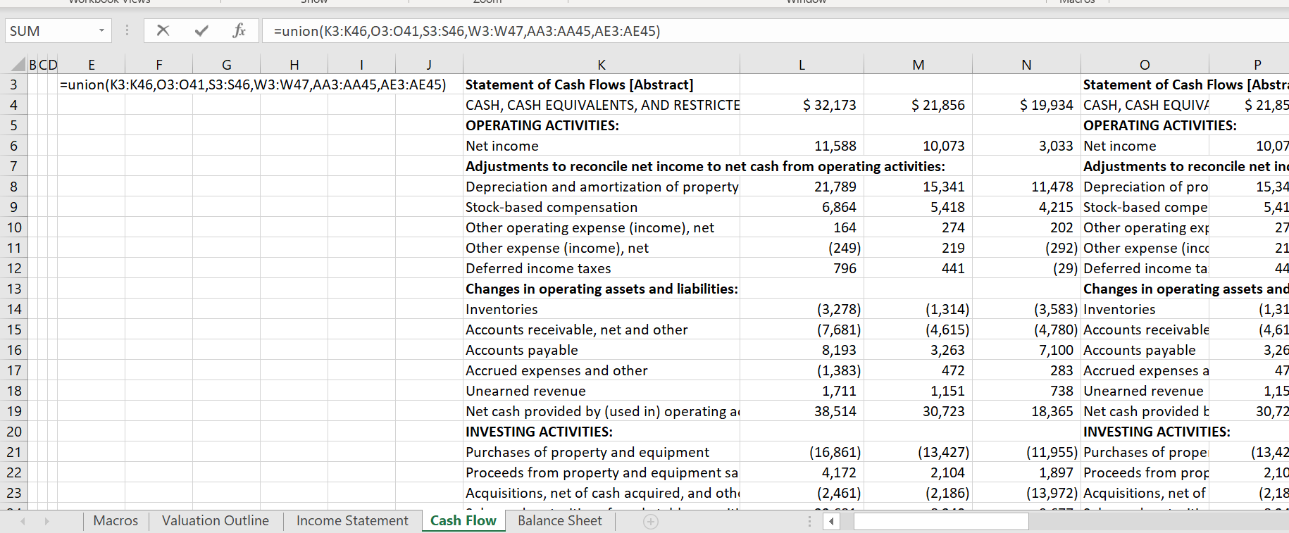
Step 2: Use the Union Function which is an array function (SHIFT, CNTL, ENTER).
Don’t forget to make enough space for a long list of columns. The argument for the UNION function is the different titles for the stuff the you read in. The use of the UNION function is illustrated in the screenshot below.
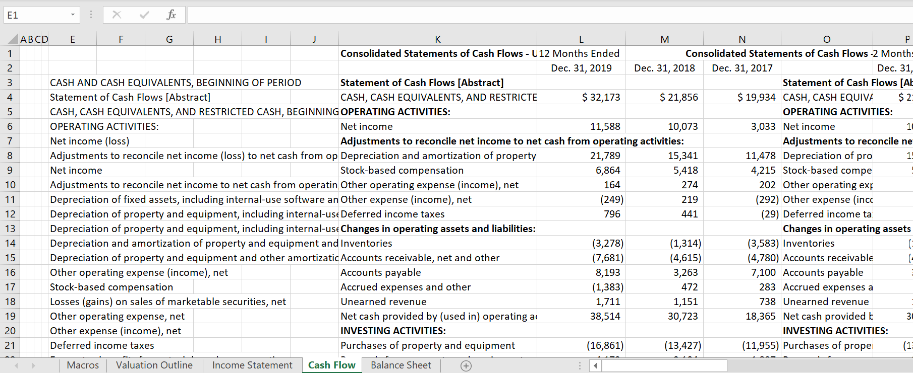
Step 3 Clean up the Union Function Output.
The union function does not always put things in a nice order. So you can copy and paste special as values, the titles and then move then around. The screenshot below illustrates the union function output before it has been cleaned up. Note that there are two titles for income. You can put these titles together and clean up the top stuff. The second screenshot shows the cleaned up version. Also get rid of the zeros at the end.
Step 4: Use the IDMAT (Index and match) to put together year by year date
You apply the INDMAT function, from the adjusted UNION function list. You compare the master list with the year by year lists and then collect the data. The INDMAT is illustrated in the screenshot below. When you use the INDMAT, use the entire row for the title of the individual year and use the entire rpw of data. As you proceed with more columns you can group (temporary hide) columns that you have finished with using SHIFT, ALT, –>. The finished result after the INDMAT is illustrated in the second screenshot below.
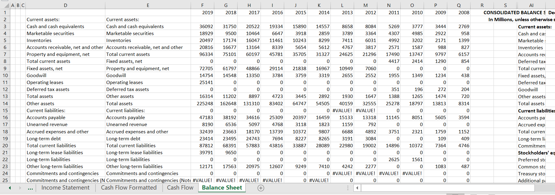
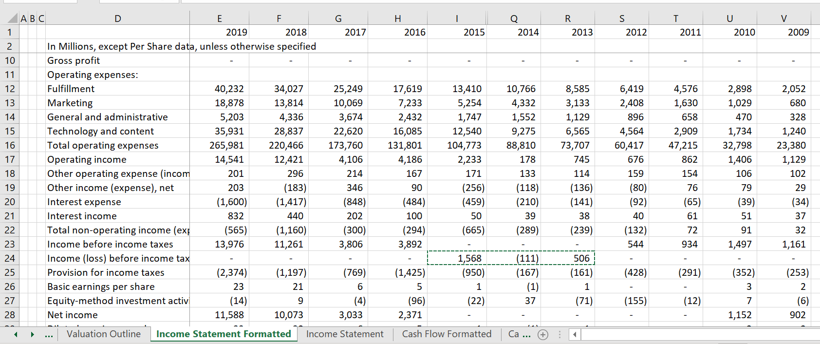
Step 5: Clean Up the Data with Multiple Rows
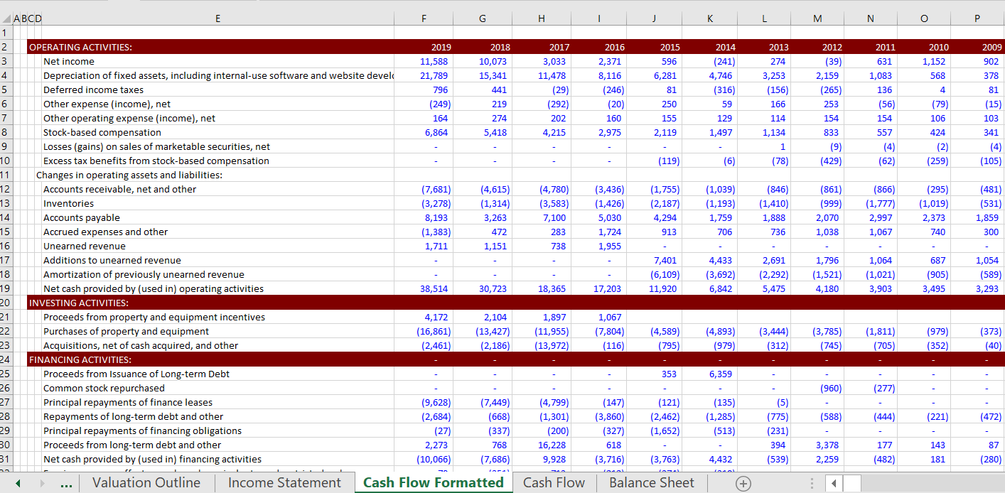
Once you have finished with the INDMAT, it will look a bit messy as shown in the screenshot below. But you can insert some columns (to save the original stuff for future years). Then you can copy and paste the information to the blank columns (or even a blank sheet). The final column will finally look clean and you have a lot of valuable history. The result is shown in the second screenshot.
The insert below shows the code for creating the INDMAT Function. You can copy this function to your sheets like for the other functions.
Function indmat(lookup_value, master_list, values) As Single ' This function does the index and match together

Dim num As Single
num = 150

For i = 1 To num ' loop around a given number
If lookup_value = master_list(i) Then
indmat = values(i)
Exit Function
End If
Next i

' On Error GoTo no_value:
' match1 = WorksheetFunction.Match(lookup_value, master_list, 0)
' indmat = WorksheetFunction.Index(values, match1)

' Exit Function
no_value:
indmat = 0

End Function