This page discusses how to set-up and structure the valuation section of a corporate model. Subjects covered include setting-up time lines and switches for the holding period and the terminal period; computing normalised cash flow in the terminal year for establishing terminal value; computing value using alternative terminal value methods including stable growth, EV/EBITDA multiples and the value driver method; evaluating the bridge between enterprise value and equity value; and applying a 1/2 year convention in discounting cash flow. The page covers a terminal value method that corrects for errors that arise by applying the formula suggested by McKinsey: Value = NOPAT * (1-g/ROIC)/(WACC-g). You can download a valuation exercise file that works through the structure of a valuation section of a corporate model by clicking on the button below. The exercises that you can work through on page named “HT Media Model Valuation”. Alternatively, you can download the file with the completed equations and look at the same page. You work either with the file with the completed analysis or the file that I made which has blanks so that you can work through some of the key acquisition modelling equations.
Summary of Valuation Crimes and Ideas
I have made the point that valuation practices are more like magic potion and visiting a fortune teller than anything resembling science. I think that the biggest crime you can make in valuation is applying some kind of standard formula for terminal value, cost of capital (e.g. CAPM with de-leveraging and re-leveraging), and comparison of multiples without understanding what is behind the formula. I have separated some points about valuation and what is behind the various sections into three sections: (1) fundamental valuation formulas; (2) intermediate valuation concepts; and, (3) advanced ideas.

Fundamentals
- Understand that the idea of a company becoming some kind of stable entity in an equilibrium is a philosophic idea and will never happen.
- Apply a 1/2 year convention should be made for both the explicit period and the terminal value; otherwise you are assuming that all revenues, capital expenditures and expenses occur at one day on 31 December. You can use (1+WACC)^.5.
- Use switches in your valuation analysis so you evaluate the sensitivity of your results to different explicit periods and terminal dates.
- Realise that a very wide range in valuation from difference is WACC is supposed to happen because small differences in return lead to big differences in money as demonstrated by stock price analysis.
- Do not have some silly idea that too much of the value in a model comes from terminal value and not enough comes from the explicit period. Think of investing your money in a stock and getting dividends and capital gains; it is the capital gain — the terminal value — that matters.
- The big number that should be used to test a model is the ROIC in the terminal period. An aggressive assumption for the terminal period will distort your valuation.
- When you change growth in the terminal cash flow a lot of other things should change, including working capital changes and capital expenditures. You can use the formula WC change = WC/EBITDA x EBITDA * terminal growth/(1+terminal growth) for working capital changes. At a minimum, the capital expenditures should be set to depreciation.
- Understand that small changes in WACC from B.S. country risk premiums and/or for small country risk premiums can have a large impact on value.
- All items in the Enterprise value to equity value bridge and in WACC should be at market value and not at book value.
- Remember that the WACC should be computed with net debt and not gross debt and the cost of cash should be the return earned on cash and other long-term investments.
- Understand that when you apply multiples, that the multiple depends on increasing or decreasing returns and changing growth rates. This is why multiples can change so much over time.
- Terminal growth should be consistent with the WACC in terms of inflation and the risk free rate.
Intermediate
- When using multiples, put the ROIC and the growth rate next to the multiple so that you can see which multiples are extreme and why. Try to find companies with similar ROIC prospects, growth rates and risks as the company being valued.
- Understand what should be in the free cash flow and what should be in the equity value to enterprise value. For example deferred tax changes from capital expenditures should be part of the cash flow calculation and not a liability in the EV to Equity value bridge.
- Realise when you should apply project finance and corporate finance principles including IRR versus ROI. When assets are lumpy for a corporation and they age, the ROI increases because of higher accumulated depreciation, but when the assets are replaced, the ROI will decline.
- Realise there are problems with ROIC from impairment write-offs, asset sales and re-structuring charges as well as service businesses. Service business can have extremely high ROIC’s and you cannot use ROI principles to gauge value; when companies have a big write-off the ROIC will increase but that does not mean the company is performing better.
- You can compute the effect of stock options granted to management with the direct amount that is paid and part of EBITDA and use base shares rather than diluted shares.
- You should adjust the terminal cash flow for capital investment consistent with different terminal growth assumptions. With higher terminal growth, you need higher capital expenditures to depreciation factors to support the graph and this factor should be in the terminal cash flow.
- If you compute Beta’s on an un-levered basis and then re-lever the beta, the debt beta as well as the equity beta should be included in the analysis. Higher debt betas can make the equity beta decrease and the equity cost of capital be less than the debt cost of capital.
- Understand the difference between applying the value driver formula with a sudden change or with a gradual change. With a sudden change, the ROIC immediately is reduced. This can address the aging plant issues discussed above.
Advanced
- Use of interpolation with ROIC changing over time per a specific definition of ROIC rather than using the value driver formula with an undefined change in ROIC over time.
- Cost of capital from market to book ratio regression recognizing that when the price to book is 1.0, the cost of capital is the same as the ROE.
- Incorporate the correct tax shield in the WACC where you adjust the percent in the capital structure rather than multiplying the interest rate by one minus the tax rate.
- Applying theoretical multiples in terminal value where you adjust the multiples for depreciation rates; for growth rates and for stable ROIC
- Adjust stable capital expenditure to depreciation factor that is discussed above along with the stable capital deferred tax for historic growth
Setting-up Valuation Switches
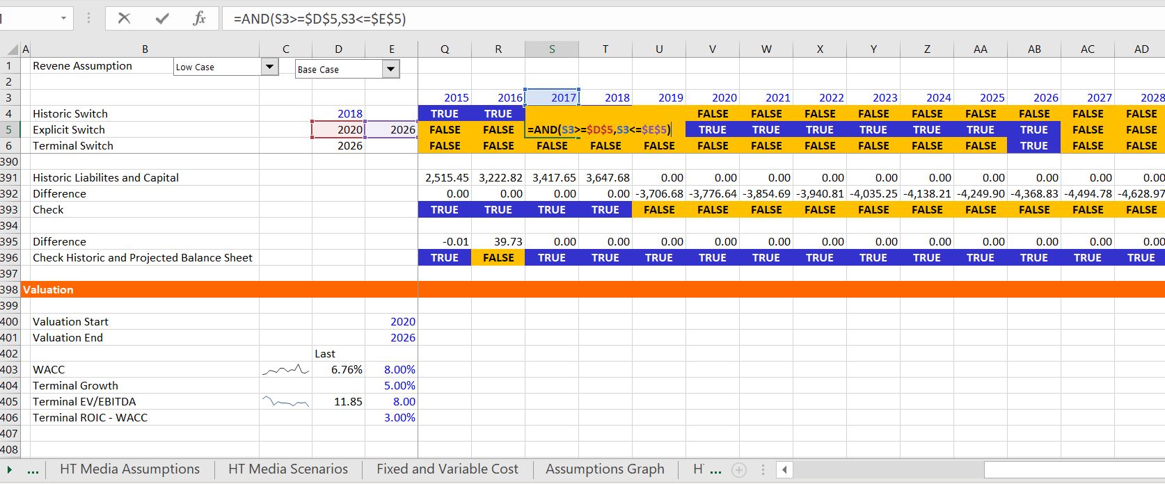
When developing a model with historic periods, you do not want to begin the valuation in the historic period, but instead a some time after the historic period. Further, you may want to consider different periods of explicit valuation cash flow — the period before which the company becomes some kind of stable boring and low growth company. I have no idea how you could possibly know this, but there is no other real option because the alternatives involve having a high rate of growth forever and/or a high return forever. So, you can enter an explicit period as shown in the screenshot below. Finally, the terminal value should be the highest amount in the valuation and the terminal year is by far the most important year (you should put the ROIC in the terminal year in your model so you can check the reasonableness of your model). In the screenshot below I illustrate calculation of explicit period switch and the terminal switch to make your model flexible. The terminal switch is really easy. You just put in the terminal year to the left and then you compare the year with the terminal year: year = terminal year. Then, you can enter the explicit period switch with the AND function. When using the AND function, refer to the year twice. The formula is: switch = AND(year>=valuation year, year <= terminal year).

Valuation Inputs and Stable Capital Expenditure to Depreciation with UDF
The screenshot above shows the required inputs for computing value using different techniques. These inputs include the WACC, the terminal growth and possibly the terminal growth, the terminal EV/EBITDA ratio, the premium between the ROIC and the WACC over the long-term; and the stable ratio of capital expenditures to depreciation that depend on the plant life and the terminal growth. This last factor is the trickiest factor to evaluate. It measures the level of capital expenditures that are required to replace exiting equipment and also to grow the company. You can see details of how this is computed in the web page that is linked to this sentence. To compute the amount, you can copy the UDF below into your file (ALT, F8, create a new macro, and paste to the top of the page to assure that Option Base 1 is at the top of the page). With the UDF you can see that more capital expenditures are required when the terminal growth is higher — the most fundamental idea in finance and in life; that you have to make an investment to get something more in the future.

.
Option Base 1
Function cap_exp_depreciation_simple(life, growth, Optional timing_code)

If IsMissing(timing_code) Then timing_code = 1

base_capexp = 100
capexp = 100

plant_balance = 100

For i = 2 To life + 1

capexp = capexp * (1 + growth) ' Capital Expenditure After Depreciation
If i = life + 1 Then retirement = base_capexp

If timing_code = 3 Or timing_code = 2 Then _
    plant_balance = plant_balance + capexp - retirement ' Closing Balances

depreciation_exp = plant_balance / life ' Depreciation on Opening Balance
If timing_code = 2 Then depreciation_exp = (plant_balance - (capexp - retirement) / 2) / life ' Depreciation on Opening Balance


If timing_code = 1 Then plant_balance = plant_balance + capexp ' Closing Balances

Next i

cap_exp_depreciation_simple = capexp / depreciation_exp


End Function

.
.
Computing Value Over the Explicit Period
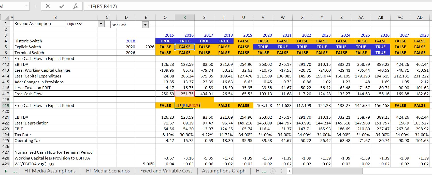
Once the inputs are established, the cash flow over the explicit period and the value over the explicit period can be computed as shown on the screenshot below. When making this calculation, you will hopefully see the utility of using the explicit switch. The free cash flow includes changes in provisions and if there were deferred taxes related to capital expenditures, these should also be included. However deferred taxes related to a net operating loss should not be included unless the deferred taxes completely reverse over the explicit period. I have put a lot more discussion on what cash flows should be included in the free cash flow versus what cash flow should be in the equity value to enterprise value (net debt) calculation in a separate web page that is linked to this sentence. In the screenshot below you see that I do not multiply the explicit cash flow by the explicit switch but instead I use and IF statement. This is important because of discounting with the NPV formula. In this case, zero is very different from FALSE. With a zero, the discounting begins in the first period with zeros when you use the entire row in the NPV formula. With FALSE, the discounting does not begin until the numbers start.
Computing Stable Cash Flow with Terminal Growth
This section discusses how to compute stable normalised cash flow in the terminal period. There are a number of adjustments that can be made to the cash flows from the model to reflect normalised cash flow. Two of the obvious adjustments include the changes in working capital and the capital expenditures. To understand the terminal value adjustments remember that you are assuming that the company will last forever and continue to grow at a stable rate. If the company’s EBITDA grows, there must be investments in inventories, accounts receivable, capital expenditures and other items that are consistent with this growth. In the case of working capital changes, if the company is assumed to grow quickly in the explicit period, but slowly in the forever period, then an adjustment must be made to reflect the changes in growth. In the explicit period, a lot of working capital investment is deducted from cash flow, but this will change dramatically in the projected period. To reflect the new working capital investment, you can use the formula: WC change in normalised cash flow = EBITDA x WC/EBITDA * g/(1+g). In the case of capital expenditures, the same sort of adjustment should be made but there is no really easy formula. Instead, you can use the stable capital expenditures to depreciation discussed above to reflect the capital expenditures that are necessary to replace equipment and also increase EBITDA by the terminal growth. The final factor that you could adjust for is the stable ROIC. This is discussed below in the terminal value section where I differentiate between two different ways to compute terminal value with the value driver method.

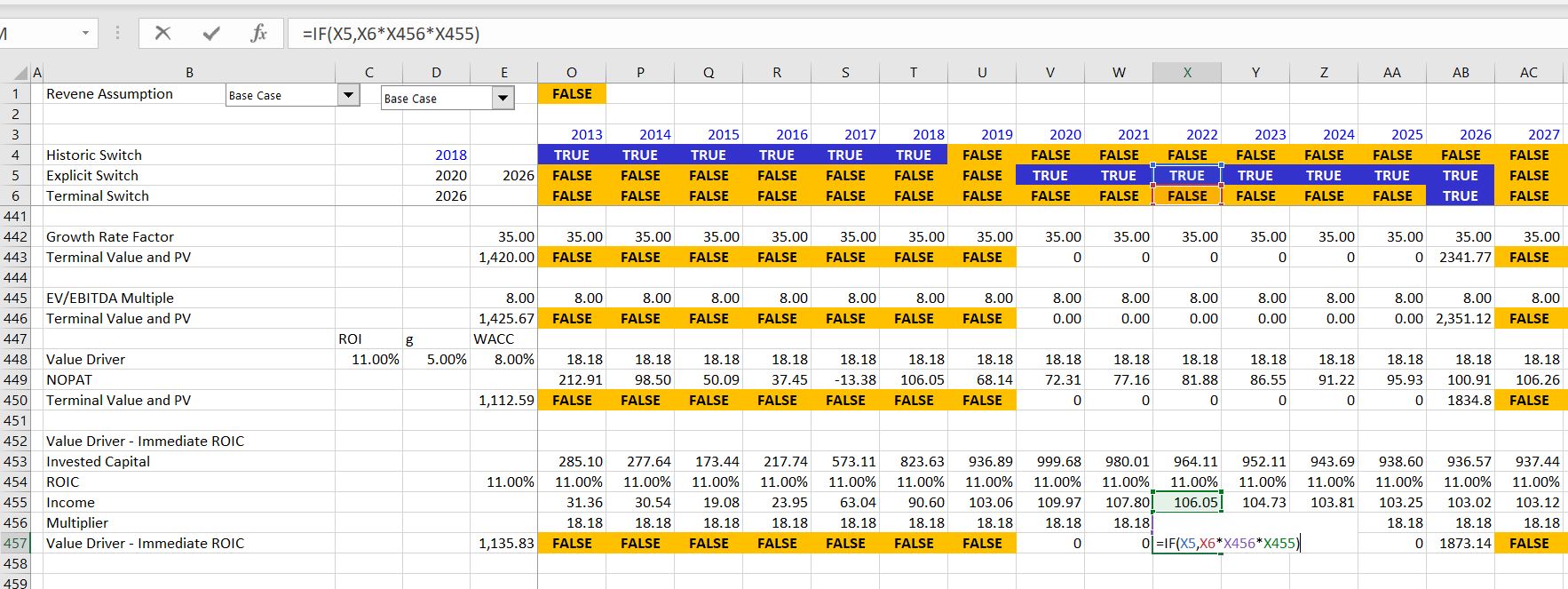
Terminal Value Using Different Methods
Computing the terminal value using different methods is discussed in this section. Five different methods are addressed and presented in the screenshot below. The first three are pretty easy and standard. These include the growth method (sometimes called the Gordon method, but I don’t like what Gordon did). The second method applies a valuation multiple, generally the EV/EBITDA and the third method uses the value driver formula where value = NOPAT * (1+g) * (1-g/ROIC)/(WACC-g). Two other methods that fix problems with the last value driver method are also included. The fourth method computes value assuming that the stable ROIC is immediately reached in the terminal year. This method uses the formula value = Invested Capital * ROIC * (1+g) * (1-g/ROIC)/(WACC-g). The difference between the two methods is that this assumes the stable ROIC is immediately met. The final method assumes a gradual change in ROIC moving from the current ROIC to a stable ROIC. This method uses the interpolate function and changes in the invested capital that are consistent with the terminal growth rate. As shown in the screenshot, this last method is more involved, but most consistent with financial theory. To implement the method, add another time line and a table for the progression of ROIC from the last explicit period down to the stable ROIC. Then compute the growth in the invested capital using the terminal growth to increase the invested capital. Next, apply the interpolate UDF function to compute the progression in the ROIC. The interpolate function is explained in the web page that is linked to this sentence. Finally, compute the ultimate terminal value in the year when the ROIC finally reaches its stable value. The second screenshot below illustrates this more complex formula which corrects for distortions in the value driver formula and allows you to explicitly think about how the ROIC may reach its stable value.
Enterprise Value to Equity Value Bridge (Sometimes Called Net Debt)
The valuation analysis discussed above only accounts for core assets and not what happens to equity value. Items that should be reflected in the enterprise value to equity value bridge can be identified by the column of 1’s and -1’s that are associated with the financing method of invested capital as illustrated on the first screenshot below. All of the items except for the equity should be reflected at the market value in the enterprise value to equity value bridge. Further, each of these items should be valued at market value and not book value. Note that provisions are not included as part of the equity value to enterprise value bridge, but investments are included if the cash flow from the investments is not part of the free cash flow. To implement the method, you can put the year before the first explicit period somewhere and then use the LOOKUP function with the projected balance sheet to find the items. In this way you can change all of the explicit periods around. To get an idea about what the relationship between the market value and the book value is, you can go back to calculation of the average interest rate and the average return on investments.
Summary of Values from Different Methods
The screenshot below illustrates results of different terminal value methods in terms of Enterprise Value, EV/EBITDA, Equity Value and the P/E Ratio. This
