It is remarkable that excel does not have an interpolate function. You can search the internet and find a couple of interpolate user defined functions (and pay), or you can use the interpolate function that is available for download below at no charge. The interpolate UDF works very much like the lookup function but it allows you to have numbers that gradually increase or decrease rather than moving in steps. You can use the interpolate function with either compound growth interpolation or with straight line interpolation.
This page explains how to use the interpolate function and the technical details of how to make the user defined function yourself. To understand the interpolate function, you should first know that the LOOKUP function is better than VLOOKUP, HLOOKUP or MATCH and INDEX. You typically lookup on a date, then click on an entire row or columns of dates that correspond to you input. You then finally click on an entire row or column of values that correspond to the dates. When using the LOOKUP function it almost seems obvious that there should be an interpolate option so values in the intermediate periods are filled in. On this page I walk through how to use and create an interpolate function after discussing the dynamic goal seek function method.
Implementation of the LOOKUP INTERPOLATE Function
To use the interpolate function you should download the file below which contains the function and some examples of how the function can be used. There are in fact two versions of the function that allow you to interpolate in different ways. The first interpolate function uses a compound growth method. The compound growth rate between an interval is computed. This compound growth rate is applied to the interval.
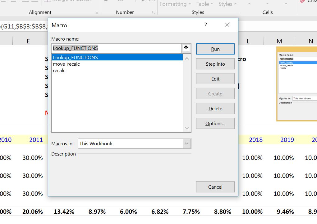
To implement the interpolate function, first download the file below. Once you open the file you have to copy the UDF function from this sheet to your sheet. To do this you can press the ALT and F8 keys to get the list of macros. Then you copy the entire contents of what is in the Lookup_functions VBA module to a module in your workbook. An illustration of pressing the ALT and F8 key is shown below. After this you edit the module; then press ALT A to select everything; then ALT C to copy everything; then go to your workbook and either enter a new module or go to the top of an exiting one; then press CNTL V to paste everything.
Once you have followed the implementation process described above, you can enter the function in your spreadsheet similar to other functions. The only difference is that the arguments for the function are not shown automatically with a user defined function. Instead, you can press SHIFT and F3 to show the required arguments. Using the interpolate_lookup function with the growth method for interpolation is illustrated in the screen shot below (the difference between the growth method and the linear method is explained below. If you look at the screen shot, the line titled ROIC uses the LOOKUP function that is described in detail in the basic function page of the website.
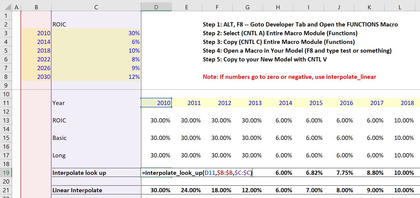
The second screenshot shows the equation of an interpolation where the amounts between the two values are divided into equal increments rather than using a growth rate method. This results in larger changes in the early part of the interpolation and lower changes later on. To apply the linear interpolation, you can use the same process with a function named interpolate_look_up_linear.
Pasting the Interpolate Function into Your Sheet
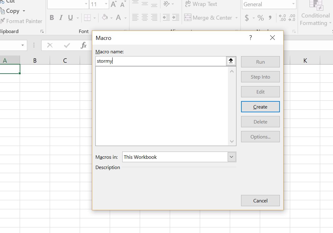
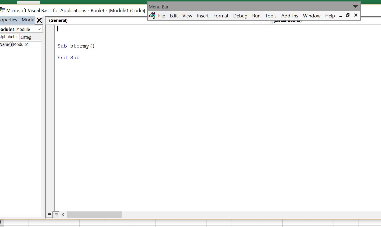
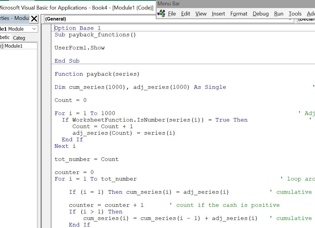
Once you have copied the VBA code (either from the userform, from pressing ALT, F8 and copying the entire sheet or from copying the code below), you can copy it into your file. To do this, you can press ALT, F8 to get the VBA screen. Then put in any name (e.g. Stormy). Then go to the top of the file and copy the code (CNTL, V). Some of this is demonstrated in the couple of screenshots below. The first screen shot illustrates how to create a new VBA page after you press ALT, F8; the second shows how you should insert a line to put the code at the top of the page; the third shows the results after you copy.
After making the new page with you blank macro named Stormy, go above the new macro and enter a couple of blank lines. When you have entered the blank lines you will press the CNTL, V and copy the code to the top of the page.
After you have copied the code into your sheet, you should see OPTION BASE 1 at the top of the page. Now you are ready to go and the function should work in your workbook.
Copy the Interpolate Function Directly from Here
Alternatively, if you just want to try copying the interpolate function from here, you can copy the code below into your spreadsheet. To do this, press the ALT, F8 sequence to see the list of macros. Then type in some new name (e.g. STORMY). Then, press the CREATE button and make sure that your new function is at the top of the page. Once you have the function defined, copy the code below to the TOP of the VBA page. In particular, make sure the OPTION BASE 1 is at the top of the page.
.
Option Base 1


Function interpolate_look_up(lookup_value, lookup_series, value_series, Optional on_off)

 Dim lookup_ser(1000) ' Allow for 1000 values
 Dim value_ser(1000) ' These dimensions are for finding numbers

 If IsMissing(on_off) Then on_off = True
 If on_off = False Then Exit Function

 max_series = WorksheetFunction.Max(lookup_series) ' find the maximum year etc. -- the key for lookup
 tot_count = WorksheetFunction.Match(max_series, lookup_series, 0) ' use the max to count how many in the series

 Count = 1
 For i = 1 To tot_count ' make a new array that only uses the series in case clicked on entire row
    If WorksheetFunction.IsNumber(lookup_series(i)) Then ' use to find the numbers
    lookup_ser(Count) = lookup_series(i) ' find the look up value
    value_ser(Count) = value_series(i) ' two new arrays that have counts from 1 to Count -- lookup_ser and value_ser
    Count = Count + 1
 End If
 Next i

 Count = Count - 1

 For i = 1 To Count ' go around counted

 If lookup_value = lookup_ser(i) Then ' If the year looking up (or date,no etc) is equal to a number -- dont interpolate
    interpolate_look_up = value_ser(i) ' If there is an exact match with then put in the number and skip rest
    Exit Function
 End If

 If lookup_value < lookup_ser(i + 1) Then ' When the year is less than the next year that read and adjusted

      If value_ser(i) <> 0 Then ratio = value_ser(i + 1) / value_ser(i) ' ratio is the current next value divided by next value

      numerator = lookup_value - lookup_ser(i) ' this is a number like 2018 - 2016

      num_of_periods = lookup_ser(i + 1) - lookup_ser(i) ' this is the total -- nothing to do with the current year in model

      If num_of_periods <> 0 Then num_raise = numerator / num_of_periods ' how much should raise to the power for interpolating

      compound_fac = WorksheetFunction.Power(ratio, num_raise) ' need to use the power function to compute compound growth

      interpolate_look_up = value_ser(i) * compound_fac ' final value of the function -- initial value x compound ratio

 Exit Function
 End If

 If lookup_value > lookup_series(tot_count) Then
 interpolate_look_up = value_series(tot_count)
 Exit Function
 End If

 Next i

interpolate_look_up = value_series(Count)

End Function
.
If you want to put the interpolate function with a linear instead of compound growth, you can download the alternative VBA code below. This code contains the different equations to make the increment equal between time periods. As with the other code, all you have to do is copy this into your file.
.
Option Base 1

Function interpolate_look_up_linear(lookup_value, lookup_series, value_series, Optional on_off)

Dim lookup_ser(1000)
 Dim value_ser(1000)

If IsMissing(on_off) Then on_off = True
 If on_off = False Then Exit Function

If lookup_value < lookup_series(1) Then
 interpolate_look_up_linear = value_series(1)
 Exit Function
End If

max_series = WorksheetFunction.Max(lookup_series)
tot_count = WorksheetFunction.Match(max_series, lookup_series, 0)

Count = 1
For i = 1 To tot_count
    If WorksheetFunction.IsNumber(lookup_series(i)) Then
      lookup_ser(Count) = lookup_series(i)
      value_ser(Count) = value_series(i)
      Count = Count + 1
     End If
Next i
Count = Count - 1

For i = 1 To Count
 If lookup_value = lookup_ser(i) Then ' lookup_value is current number for year etc (e.g. 10)
    interpolate_look_up_linear = value_ser(i) ' if the look_up value is the same as a value in table set to value
    Exit Function
 End If
 If lookup_value < lookup_ser(i + 1) Then ' case where the look up value is less than the last one
    num_difference = lookup_ser(i + 1) - lookup_ser(i) ' find the difference in total years for the denominator
    val_difference = value_ser(i + 1) - value_ser(i) ' difference in total values for numerator
    If num_difference <> 0 Then increment = val_difference / num_difference

    num_of_increments = lookup_value - lookup_ser(i) ' total number of increments from start
    total_adder = num_of_increments * increment

    interpolate_look_up_linear = value_ser(i) + total_adder
    Exit Function
 End If
 If lookup_value > lookup_series(tot_count) Then
    interpolate_look_up_linear = value_series(tot_count)
    Exit Function
 End If

Next i
interpolate_look_up_linear = value_ser(i - 1)
End Function
.
Interpolating without a Function
Many people interpolate in excel without a function. This can be done with the GROWTH function in excel using a few steps or you can compute the compound growth rate by yourself. This is a painful process for something that should be automatic and of course I don’t think this is a very good idea. For some reason when I made the not very good video below that describes this process I recieved a lot of views.
Video that introduces the macro process with cells.select
[wonderplugin_video iframe=”https://www.youtube.com/watch?v=3ArFFHZXI0g” videowidth=600 videoheight=400 keepaspectratio=1 videocss=”position:relative;display:block;background-color:#000;overflow:hidden;max-width:100%;margin:0 auto;” playbutton=”https://edbodmer.com/wp-content/plugins/wonderplugin-video-embed/engine/playvideo-64-64-0.png”]
Making a Lookup function with Na like the false
Re-Creating the LOOKUP function to Introduce the Technical Process
Lookup_NA.xlsm
This video introduces the technical process through explaining how to make your own LOOKUP function. But when re-creating the LOOKUP function you can design it so the nasty NA does not appear when there are no values associated with one of your dates (or key values). For example if you model starts in 2018 and you start your look-up values in 2019, the excel lookup will put in NA. You can write your own function to put in a FALSE instead of an NA which will cause a whole lot less problems when you are making a model.
[wonderplugin_video iframe=”https://www.youtube.com/watch?v=oVBLRPmaE3M” videowidth=600 videoheight=400 keepaspectratio=1 videocss=”position:relative;display:block;background-color:#000;overflow:hidden;max-width:100%;margin:0 auto;” playbutton=”https://edbodmer.com/wp-content/plugins/wonderplugin-video-embed/engine/playvideo-64-64-0.png”]
.
[wonderplugin_video iframe=”https://www.youtube.com/watch?v=D9vJYvjf3i8″ videowidth=600 videoheight=400 keepaspectratio=1 videocss=”position:relative;display:block;background-color:#000;overflow:hidden;max-width:100%;margin:0 auto;” playbutton=”https://edbodmer.com/wp-content/plugins/wonderplugin-video-embed/engine/playvideo-64-64-0.png”]
.