On this page I try to discuss what it really means to have a transparent model, in particular a transparent project finance model. The over-riding issue is to keep formulas short. In discussing transparency I also address a few other issues. One aspect of transparency is keeping the drivers of a formula in your sight when you press the F2 function key. A second aspect is simply making the titles of your items very clear. A third element of transparency is using the LOOKUP, INDEX and SUMIF functions in excel and virtually nothing else except EDATE, MIN and MAX. Finally, in making things transparent, make the model flow in a nice, smooth and artistic way and do not look down for things unless you have a circular reference. If you find yourself with a long formula with other functions, go and take some kind of break or drink a glass of wine and think through it. I promise that you can make in more efficient and transparent.
Using LOOKUP with Entire Row or Column
In this section I discuss the LOOKUP function which is one of the few functions (including INDEX and SUMIF) that is really useful in your models. When using this, please be one of the few people in the world who uses the entire row or column instead of wasting time pressing the F4 to lock in ranges of cells. Also, do not think your are cool by using INDEX, MATCH; LOOKUP is far easier as long as the target cell as a continually increasing series like a date or a period counter. You could think about the LOOKUP function as LOOKUP(Target Single Cell, Row with Data Corresponding to Target Cell, Data to Plop into the Result that is in the same column as the corresponding row). I promise that this will speed up your programming and it will not make your models heavy. To illustrate application of LOOKUP, I have presented a few examples of what not to do with screenshots of models that I have tried to restructure. The first example in the screenshot below illustrates the crime of using VLOOKUP where you have to input the row number 2. The screenshot shows that people still waste time with the VLOOKUP function — if you insert a line, the whole formula breaks down.

Almost as irritating as using VLOOKUP or HLOOKUP is wasting time by pressing the F4 when creating the lookup function instead of simply clicking on an entire row or column after the target cell. This is illustrated in the next couple of screenshots. The first screenshot makes me start to shake because of the utterly useless colours. The formula shown above the sheet must have taken a long time to enter and it is not transparent. The second screenshot is almost as bad and is a typical thing that you see in models. The general rule is that when you take items from the input sheet that is expressed in time series, then you should use one single lookup function. In the lookup function, you can see the line that is used in the time series file.


An efficient use of LOOKUP is shown in the screenshot below. In this case the entire line 68 from the time series is used and the line 70 is used. This should be clear from the formula. In general, the only time that you take things from an input file that are not in the left column should come from the LOOKUP formula. When using the LOOKUP function, put a blank left column to make sure for the target cell (in the case below, in line 68) so that an NA does not result. All you have to do is put the model start date or a zero etc. in the left column of the comparative line that you will be gauging against the target cell.

Using SUMIF with Entire Row or Column
The SUMIF or SUMIFS functions are the third kind of function that should be used in an elegant manner in a model (other than LOOKUP and INDEX). The most basic use of these functions is to aggregate periodic data (monthly, quarterly or semi-annual data) into data that you can read and interpret. The screenshot below illustrates use of the SUMIF function. Note that if you lock in the rows on the detailed period sheet (in this case IFS) and you lock in the row but not the column number and do not lock in anything for the entire row, you can create an annual sheet in seconds. To create balance sheet accounts, you can use the SUMIFS function with a flag for the end of the period.

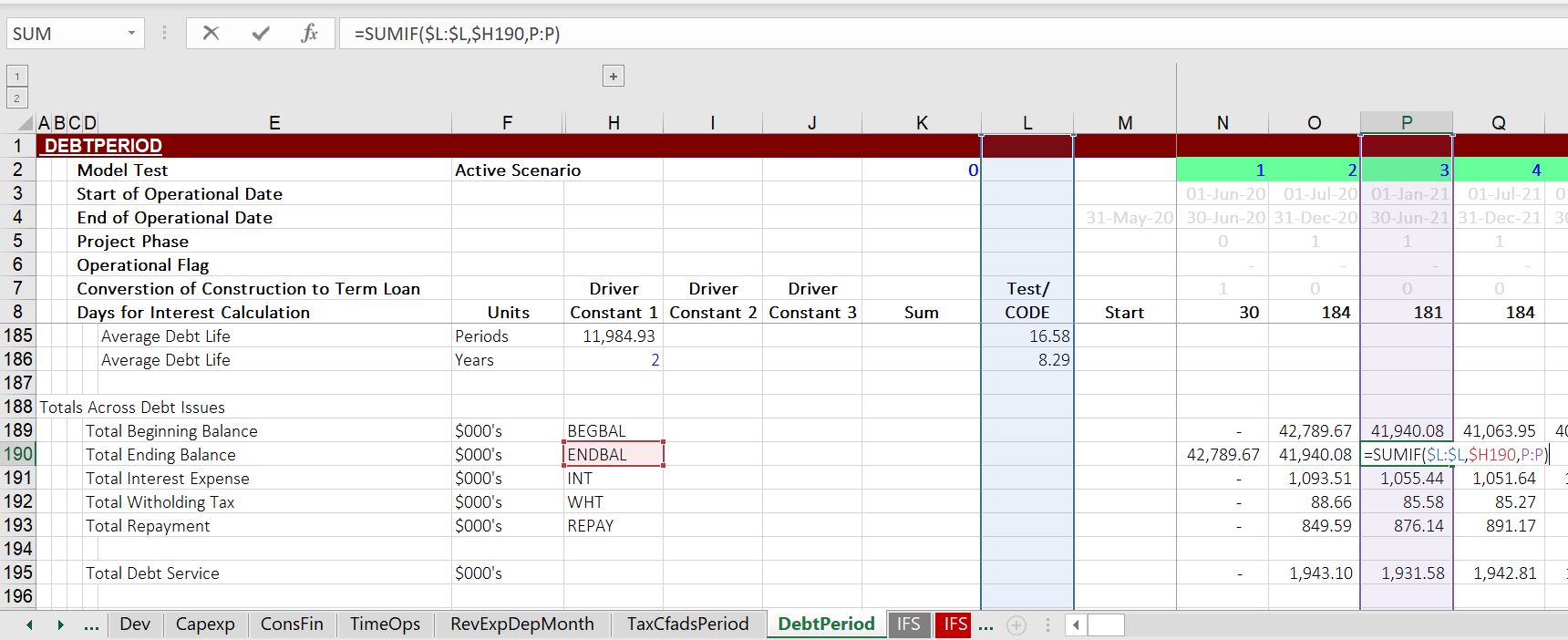
SUMIF for Aggregating Across Debt Issues
Another use of the SUMIF is to aggregate debt issues using code names. My suggestion is to not engage in the torture and dangerous simple sum functions. Instead of this, you can use the SUMIF with code names. A big use of SUMIF is for the annual totals as shown in the example below.

Why Range Names Suck
There are many reasons not to use range names. They are particularly painful when importing sheets from one file to another file and some of the range names in the two files are the same. I think they can can be used for a very few items like the unit names or maybe dividing by 12 months per year or 360 days per year. You can trace the location but it is a pain. They can result in errors as shown below.


INDEX Function and Trying to Impress with Fancy Excel Formulas
I have repeated over and over again that all you really need to do is focus on the INDEX, LOOKUP and SUMIF. You can do just about anything with these functions and you do not need many added functions. The example in the screenshot below uses OFFSET and is largely a waste of time. Why in the hell would you use the offset formula instead of a simple CHOOSE or INDEX formula. The second example the OFFSET function is used again with hourly data that is useless in a financial model.


What is Not Impressive in a Model
It is very nice that you can use the CNTL, 1 short-cut and then make the number 1 appear as yes or as “On” as shown in the example below. Isn’t it much nicer to just use TRUE and FALSE where you can even attach a check box. The same is for Yes and No below. You can make this by pressing CNTL, 1 and then go to the general section and then put in “Oui”;;”Non”.


When you use an IF statement with 1 and 0 or TRUE and false, you should realise that IF(TRUE, true condition, false condition) results in TRUE and that any number other than 0 is true. This means that when you want to test a denominator with an if statement, you can use IF (B,A/B). When B is anything other than zero, this gives you the result A/B. When B is zero, this gives you FALSE.

Useless Macros and Inconsistent Formatting
Scenarios and the INDEX Function
There are many ways to make scenarios in a model and I have an entire set of web pages discussing scenario analysis. But there are a couple of things that are very basic for any scenario analysis. First do not muck up your input sheets with a bunch of scenarios. Second, always use a code number and the INDEX function. An example of really messed scenarios is illustrated in the screenshot below.


Don’t put some sheets with vertical layout and other sheets in horizontal format.
