This page describes fundamental and advanced issues associated with the Loan Life Coverage Ratio (LLCR) and the project life coverage ration (PLCR) in project finance. The LLCR and PLCR ratios can be used to assess break-even but using different definitions as to what constitutes break-even from the standpoint of a lender and can be better than the DSCR is at its core a gauge for measuring break-even points. The LLCR that measures the ability to repay a loan over the life of the loan and can be difficult to compute if there are multiple different issues with different interest rates and different debt tenors. The LLCR is the present value of cash flow divided by the debt level at the period evaluated. The problem is what is the discount rate that should be used in computing the present of the cash flow. I argue that you should compute the prospective debt IRR when making this calculation which can be tedious without using an user defined function. An analysis demonstrating the break-even idea is presented below as well as some advanced and tricky details about computing the LLCR when there are different debt issues with different maturities and different interest rates.
The Notion of Break-even and Credit Analysis
If the cash flow available to pay debt service is 100 and the debt service is 50, then the break-even cash flow is 50, which is a decrease of 50, or 50%. In this case the DSCR is 100/50 or 2.0. The break-even percentage decline in cash flow is 50% (not 100%). The formula for finding the break-even decline in cash flow is just:
Percent Reduction in Cash Flow Flow for Single Year Default = (DSCR-1)/DSCR.
In a similar manner, the LLCR and the PLCR can be used to compute the percent decline in cash flow that can occur before a problem. In the case of LLCR, the result gives the decline in cash flow with restructuring that can occur and the loan can still be paid by the end of the loan life:
Percent Reduction in Cash Flow for Repaying Loan by end of Loan Tenor = (LLCR-1)/LLCR
Similarly, the PLCR provides the percent decline in cash flow over the entire project life that can occur and the loan can sitll be repaid in full. The difference between the LLCR and the PLCR provides the added buffer the provides safety from the tail — the difference between the end of the debt tenure and the project life. The formula for the PLCR that defines break-even can be expressed as:
Percent Reduction in Cash Flow over Entire Life for Repaying Loan = (LLCR-1)/LLCR
Definition of LLCR and PLCR in Simple Case with Individual Debt Issues
If the DSCR is CFADS/Debt Service, the PLCR puts PV factors around the CFADS and the Debt Service. But since the PV of debt service is the same as debt at COD (or after COD), the PLCR can be defined as:
PLCR = PV of CFADS over Project Life/Debt
If there is a debt service reserve account this should be subracted from debt using the principal of net debt in corporate finance (cash is like negative debt).
For the LLCR, the formula is similar but the cash flow is computed over the loan life. So the formula is:
LLCR = PV of CFADS over the Loan Life/(Debt – DSRA)
To demonstrate the break-even points, you need to make a model with a default waterfall. The file below includes a default that is repaid and demonstrates how the LLCR and PLCR measure the break-even cash flows.
PLCR and LLCR Break Even Exercise
Excel File with Stock Prices, and Economic Variables with Computation Returns and Long-term Analysis
Multiple Issues and Different Interest Rates
Lawyers can go crazy and charge a whole lot of money in defining the LLCR. I don’t really care what is written in a loan agreement. Here I show the theory of the LLCR and how it should be defined with multiple debt issues that have different interest rates. This issue arises for the Green Climate Fund that provides concessional debt financing. You can download a file that has a pretty simple example of two different issues (no circular references, no taxes, no sculpting). This file is attached to the button below.
The screenshot below begins with a single issue. In this case you can see how the LLCR works. The first screenshot has a case where there is enough cash flow to pay off debt. This is demonstrated with a cash sensitivity factor of 150%. This results in an LLCR of 1.21. Using the formula cash flow reduction = (LLCR-1)/LLCR suggest that the cash flow can fall by 17.04% as shown in the screenshot. 150% multiplied by (1-17.04%) produces 124.4%. The second screenshot shows what happens when the cash flow is reduced to 125%. Note that the LLCR is exactly equal to 1.0.


The next screenshot demonstrates what happens when the LLCR is below 1.0. In this case I have reduced the cash flow percentage to 120% which is below the LLCR implied break-even. In this case, the debt cannot be repaid over the debt life. Note that the debt can be repaid by the end of the project life because the PLCR is above 1.0. (We could be doing the same exercise with the PLCR).

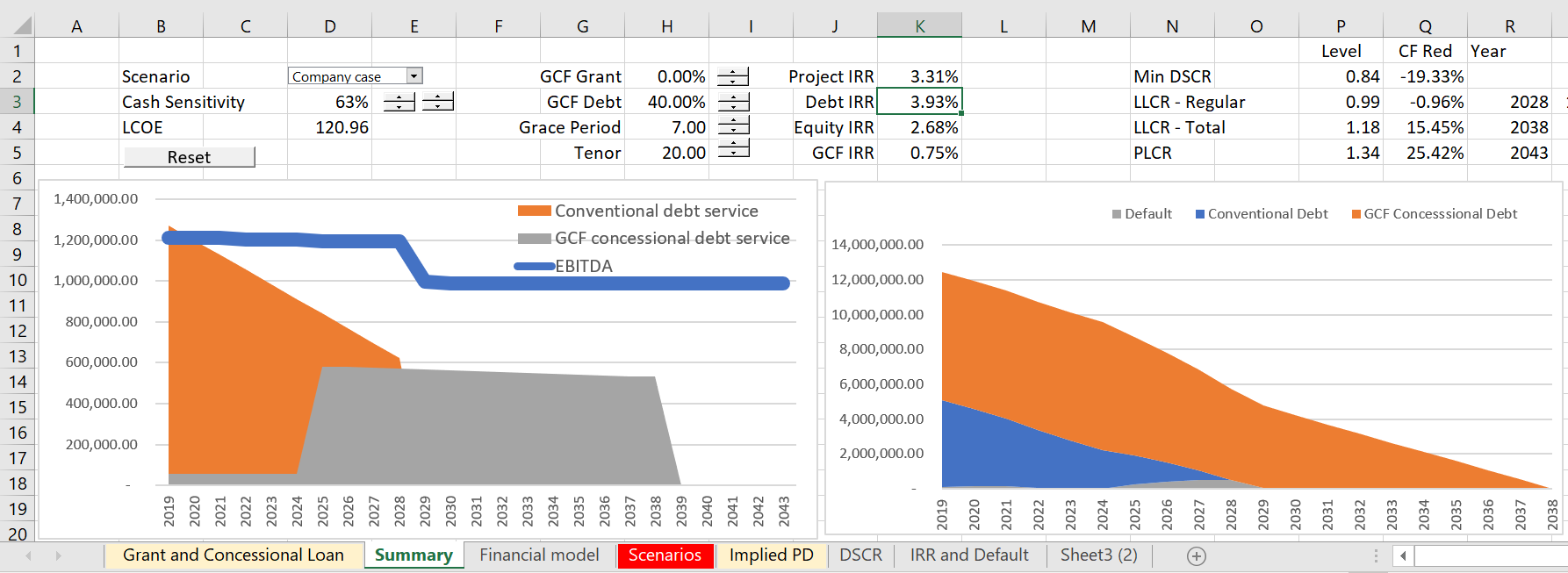
Now a second debt issue is added that has a long-tenor, a grace period and a very low interest rate. This is representative of an issue for the green climate fund. In this case you can compute the LLCR for the first regular old issue and a second LLCR for the GCF issue. For the first issue you need an interest rate for the LLCR. This can be computed from the debt IRR that combines issues and is truncated at the tenor of the first debt for the LLCR on the first debt issue. The technique for doing this shown in the screenshot below. Note that the debt IRR is actually negative. But this still works.

To demonstrate how the LLCR works in this case, I begin with a case where there is no default and the cash flow sensitivity factor is 100%. Here the LLCR is 1.57. The 1.57 implies that cash flow can decline to 63% and the first tranche of debt can still be paid by the end of its life. The second screenshot tests this out by reducing the cash flow. Note that it really does work.

More Complex LLCR Case and Video
The two files below demonstrate other issues associated with computing the LLCR. The first file demonstrates how to deal with changes in interest rates and also multiple issues. The second file demonstrates how to use the SUMPRODUCT function when the interest rate changes.
Excel File Demonstrating How to Use SUMPRODUCT Function for Changing Interest Rates