On this page I attempt to take mystery away from computing the levelized cost of electricity, the levelized cost of hydrogen or the levelized cost of just about anything else. My biggest points are: (1) you must be able to prove levelized cost with a project finance model as they are essentially the same thing (a project finance model computes IRR from price and levelized cost computes price from IRR); (2) levelized cost is an economic concept to evaluate the economics of different technologies and strategies; as such, it must be based on real costs (i.e., adjusted for inflation) and not nominal costs (Lazard makes this big error); (3) you can compute levelised cost in different ways, but the most clear method is to use the PMT function.
I demonstrate that you can compute the levelized cost using four different methods that I name (1) the carrying charge method; (2) the NPV(revenue)/NPV(generation) method; (3) the NPV(cost)/NPV(generation) method; (4) the weighted average price method. All of these methods produce the same result when you make the correct calculation and when you use a correct and consistent costs of capital. But I argue that the best way to compute levelized cost is to use the first method because you can evaluate the things that drive the levelized cost.
The idea of levelized cost is not some kind of economic analysis that is unique to the energy industry and it is not some kind of specialized measurement technique for electricity generation projects. It is just measuring the cost per unit of something on a consistent basis so that you can compare the economics between alternatives. I will emphasize in the next few pages that computing the levelized cost does require a bit of thinking about things like taxes, financing, degradation and inflation, but once you make certain calculations it is straightforward. It drives me a little crazy to look at power point slides that discuss levelized cost and make you think that the calculation of levelised cost is some kind of mysterious fancy calculation.
The levelised cost of just about anything fundamentally depends on a few variables (the same variables that drive any project finance model):
- the capital investment you make for the project;
- the fixed and variable operating costs;
- the production you will achieve from the efficiency of the machine (or horse or person) and,
- a range of financial variables associated with translating the up-front capital costs into costs over time.
In discussing the different techniques, I emphasize that the real cost without inflation rather than the nominal cost is the appropriate benchmark for comparing technologies that have different capital and operating costs. When you can measure the correct cost of something, it is a big deal. You can then evaluate business strategies that work with the most effective cost cases. For example, if you are evaluating hydrogen options, it may be better to put electrolyzers at the customer site (paying a higher price because of economies of scale), and oversize the electrolyzers so you only use solar power during sunny periods. The file that you can download by clicking the button below includes my LCOE calculator with some advanced issues related to taxes, financing, degradation, inflation and the lifetime of assets. The second file is the standard calculator without the ITC and the depreciation.
.
.
Working File for Levelised Cost of Electricity Analysis with Solar Data and LCOE Calculations
.
Excel File with Levelised Cost of Electricity Mechanics Including Detailed U.S. Tax Aspects and ITC
.
.
Principle 1: Use of PMT Formula as a Better Way to Compute Levelised Cost
Levelised cost can be computed in a couple of steps from the three inputs (Capital cost, operating cost, production) along with the life and the discount rate and the degradation rate. You can use the PMT formula which just is levelising capital costs over time. This is the fundamental definition of levelising cost. If there are no, taxes, no inflation, no degredation, then the levelised cost can be computed in the following steps:
- Capital Recovery = PMT(Discount Rate, Life, Capital Investment)
- Total Annual Cost = Capital Recovery + Operating Cost
- Levelised Cost = Total Annual Cost/Production
I received an email with the following provocative comment on LCOE:
I am surprised you have a bee in your bonnet about LCOE. The math is actually straightforward, even my fellow colleague who has a History of Arts degree from the university of southern Uzbekistan knows the math behind this. By the way most developers don’t give a rats arse about LCOE. All they care is getting their equity IRR, get out of the equity lockdown period, take the cash and use it somewhere else. Only policy makers and self-aggrandizing politicians give a hoot about LCOE.
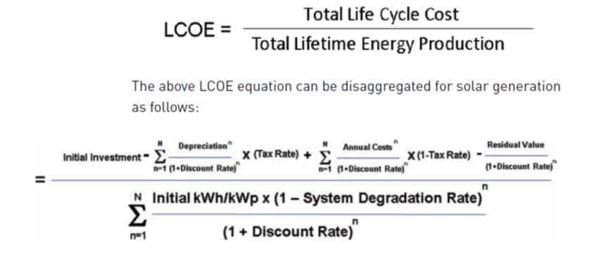
I like the way this comment is written but I must disagree. There are nuances in computing and interpreting the LCOE that are often missed and the calculations can be a little tricky. I do not see calculations that correctly account for different lives, inflation, degradation tax rates and financing very well. For example, you may see the formula below that includes residual value, adjusts annual costs of taxes and does not specify whether the discount rate is pre-tax or after-tax. Applying this formula for different lives would be a pain when you are trying to evaluate the difference between different alternatives. If the math is so easy, then why do people not know that the only way to make the formula using costs sensible is to use.
If you have varying interest rates you may have to compute the PMT function by hand. It is unfortunate but people have seem to forgot this. If you do a google search you cannot even find this. To compute it by had you can go back to the definition of PMT with a PV fromula as shown below for a on period case and a two period case. In this, the PMT is represented by x.

To apply this formula in an example, you can compute an index and use the sum function as shown below.
.

.
If you have varying discount rates because of changing inflation, changing degradation or even changing cost of capital, you can apply the PMT formula and prove it as follows. Note that the PV of PMT is computed by using the varying discount rate.
.

.
Bull Shit Formulas versus Consistent PMT Formulas in Excel
The formulas below are often used in different presentations. This is bull shit blah, blah blah. Please look at the LCOE calculator that adjusts for real costs, taxes, degradation in output; degradation in input; adjusted nominal O&M costs; alternative tax depreciation rates and other factors.
An example of using the PMT function with different adjustments is shown below. If you take the time to work through this page you will be able to see how all of these items work and you can become comfortable with the process.
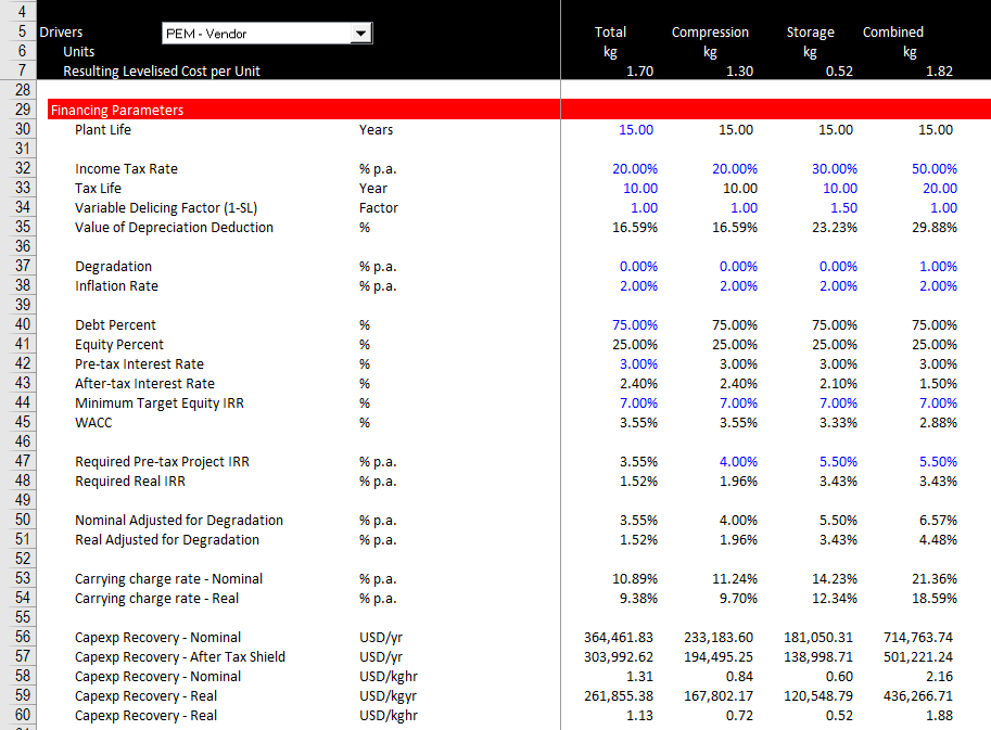
After defining the operating parameters which can be for a battery, a horse, a hydrogen electrolyzer, a truck, an airplane …., you can input some financial parameters which define how the capital costs are translated over time. Unlike the operating parameters, these parameters are similar for different projects and involve things like inflation, interest rates, plant life, gearing and taxes. Inputs for these factors are illustrated in the screenshot below.
.
.
Principle 2: Prove that a Project Finance Model Gives you the Same Results — The LCOE Gives you Price from IRR input and the Project Finance Model gives you IRR from Price
I have worked matching a project finance model and equations that use the PMT and PV functions to compute the levelised cost of electricity. The file attached to the button below includes a data set with the Lazard operating assumptions and many different financial inputs. The file demonstrates the importance of project finance in evaluating the cost structure of capital intensive investments.
.
.
LCOE is simply the complement or recriprocal of a financial model when done correctly, meaning that the inputs to the LCOE calculation are like putting factors into a financial model and then doing a goal seek to find the price. When computed correctly, the LCOE can be used to do an analysis of what strategies make most sense such as batteries and hydrogen.
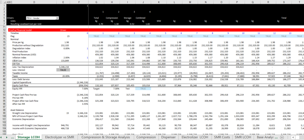
When verifying the LCOE calculations with a financial model, the after-tax project IRR should be exactly the same as the cost of capital that you input in the LCOE analysis. In the screenshot above, the real cost of capital is 3.55% after adjusting for debt and the interest tax shield. In the screenshot below, after the taxes are accounted for along with degradation, inflation and debt, the after tax project IRR in the model is the same as the 3.55% value that is input. The verification is made when you use the nominal or real LCOE as price input in the financial model.
.
.
Principle 3: Please use Real LCOE aand not Nominal LCOE and Understand the Difference
My good friends in Malaysia signed a contract to sell water to Singapore in the 1950’s and did not include inflation in the contract. This was a contract without inflation like a PPA without inflation. Now the water is absurdly cheap as a Singapore dollar in 1953 does not buy the same things as it would today. This I hope illustrates why it is essential to use real currency and not nominal currency. At least for economic analysis.
The use of real instead of nominal cost in economic analysis makes more of a difference the longer the asset life. So the hydro LCOE will be dramatically overstated if you incorrectly use nominal LCOE for the hydro plant. This is far less important for a natural gas plant where so much more of the costs are variable operating costs.
.
Principle 4: Alternative Methods including NPV of Revenues or NPV of Costs Divided by NPV of Generation Produce the Same Result
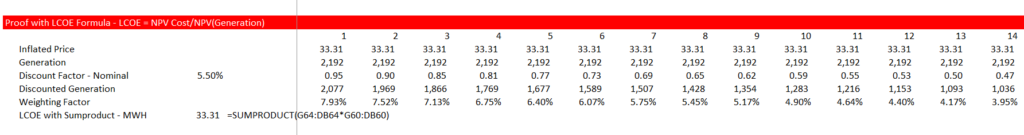
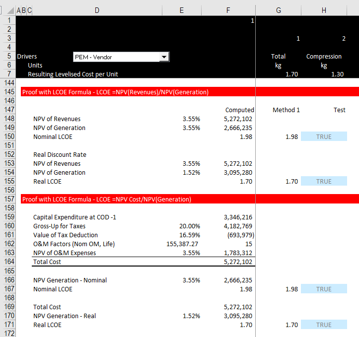
Next, you can prove the formulas for LOCE — NPV Revenues/NPV Generation and NPV cost/NPV Generation product the same result if the pre-tax IRR is used as the discount rate. The screenshot below demonstrates that the LCOE (of 213 RM/MWH) in the financial model is confirmed with the other LCOE methods.
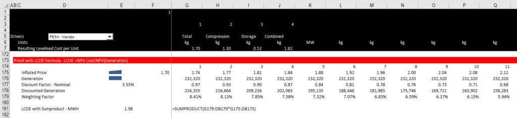
The LCOE can also be computed using with a weighted average price. This demonstrates what the levelizing really means — it is just a weighted average. The weighted average could be computed in real or nominal terms. In the screenshot below, the starting point is the real rate, but this price is escalated over time.
.
.
Videos associated with Levelized Cost
There are a series of videos that describe the various issues associated with computing levelised cost. I am sure there is one correct method to compute the levelised cost that you can prove with a project finance model that includes re-financing and terminal value. I have no idea how you could watch all of these videos without going crazy. But you may want to tak a look at a couple of them.
If you want the files associated with levelised cost I have the files in a folder (chapter 5, conventional energy) of the resources. Just drop and email to edwardbodmer@gmail.com and I will send a google drive with a whole lot of stuff (probably too much). But you can unzip the files and look for what you want and save the google drive in the cloud….
.
.
.
The videos below walk through the process and illustrate some of the details in computing levelised cost.
.
.
Excel File that with Levelised Cost per Unit Template with Case Study for Hydrogen Transport Trucks
.
Computing the Levelised Cost of Anything to Evaluate Business Strategy
When listening to a story about Beethoven, I found out that he had a horse that he did not take care of very well. Instead, he liked better to drink some cheap wine apparently while he composed the most remarkable music when he was deaf. When I heard about Beethoven’s horse I immediately thought about the levelized cost of his horse. Beethoven’s horse had a capital cost and a fixed operating cost to feed the horse even when the horse was not transporting Beethoven around (Beethoven apparently did not do well in feeding his horse). You can divide these fixed costs of the horse by the amount of distance the horse travels and then add the variable cost of feeding the horse you could compute a cost per km or the cost per km. You can even account of externalities of the horse pooping in the road.
Here’s how you can think about it quickly:
- What is the output of the investment — km, kWh, kg, bbls, MMBTU etc.
- Compute the capital cost of getting this output by making an investment
- Compute the fixed and variable costs
Once you have these numbers, you must spread the cost over the years and then over the production. You should also be careful with real and nominal costs for the operating costs. I hope this makes you can compute the levelized cost of just about anything. I suggest when making an evaluation of something like a solar project or hydrogen, you should begin with levelized cost analysis. As I could not find a picture of Beethoven’s horse, I show a picture of a garbage truck that was driven by horses. We could in theory compare the levelized cost of this to the levelised cost of a diesel truck and then a hydrogen truck.
Case 1: Simple Example with No Inflation; No Taxes; No Degradation; No Asset Replacement and Proof with Using the PMT Function
On this page I introduce a generic levelised cost calculator where I hope you can fill in capital costs, operating costs, efficiencies along with some financial parameters to easily compute the levelised cost. You will never be beholden to a Lazard website or a fancy power point presentation that does not explain where things come from. To explain the carrying charge method (which I advocate), I use the following step by step process:
- No Inflation, no taxes, no degradation, no debt financing — just use the PMT function without adjustment
- Add inflation — Use the PMT with a real discount rate and use the PV function to adjust O&M expenses when computing nominal LCOE
- Add degradation — Use the PMT function with real and degradation adjusted discount rate; make an adjustment to the real and nominal O&M expenses using the PV formula
- Add debt to the analysis — Create a project finance model and use a goal seek to derive the project IRR or use the WACC and demonstrate the result with economic depreciation
- Add taxes to the analysis — compute the PV of the tax shield and adjust the PMT formulas by dividing the PMT by (1-tax rate).
This excel sheet computes levelised cost from your defined inputs for capital costs, operating costs and amount of production. The program then ties the levelised cost calculation to a simple financial model and proves that the target return in the levelised cost parameters is equal to the resulting equity IRR in the financial model. You can download the financial model by clicking on button below. The example also assumes no inflation and is computed on a nominal basis. With no inflation and no degradation, the revenues and the price and the generation is constant. You can compute the present value of revenues and then use the PMT function.
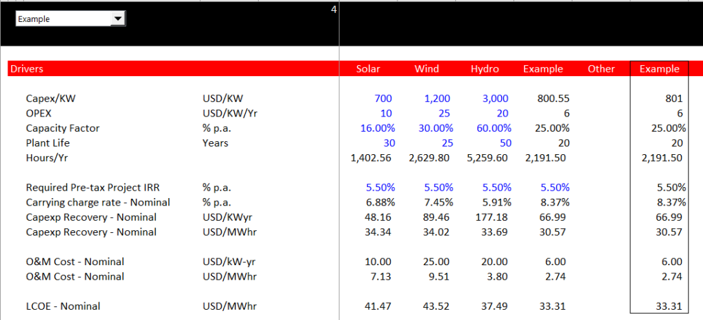
In the example below you just need to know how to use the PMT function to compute the carrying charge. This is in line 21 where the PMT function is computed from the capital cost. Here the formula is PMT(Discount Rate, Life, – Capital Cost). Then you can compute the annual costs by adding the fixed costs and divide them by the kWh production. You can clearly see the drivers of the cost.
Proving the Simple Case (No Inflation, No Degradation, No Taxes) with a Financial Model
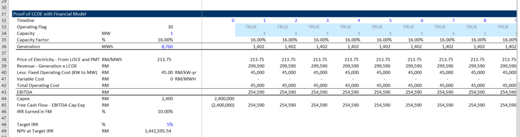
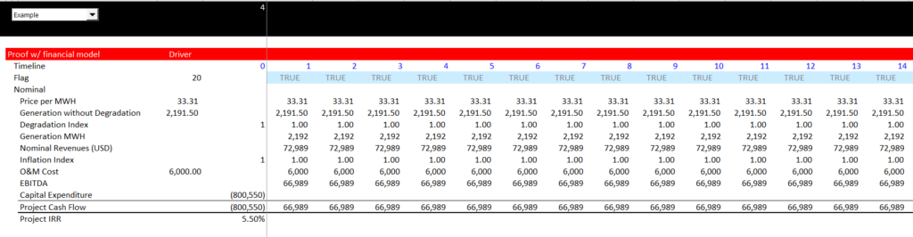
Once you have the LCOE you can prove that it really works with a simple financial model. The financial model involves computing a time line from the life of the project and then developing a couple of equations for the amount of production from the capacity of the project. The example below is for an electricity project and the production is MWH.
After you have computed the generation, you can compute the revenues from the price and quantity. The key is to use the LCOE you computed with the PMT functions from the prior section as the price. You can then drop in the operating costs and the capital costs to develop the free cash flow. With the cash flow, you can compute the project IRR. This project IRR should be the same as the cost of capital that you input. This is the fundamental chech of the model and the idea should be the same once you add more complex items like degradation, taxes and
Case 4: Inclusion of Income Taxes and Tax Depreciation
The next section evaluates levelised cost when the quantity of the units change. Different amount of units affects the weighting of the levelised price. For example, if the number of units is half of the units when the units start and if the price changes, then weighted average price changes. Without discounting, the screenshot below is 13.33.
More Details on Solar Nominal Levelised Cost without Degradation, Taxes or Debt
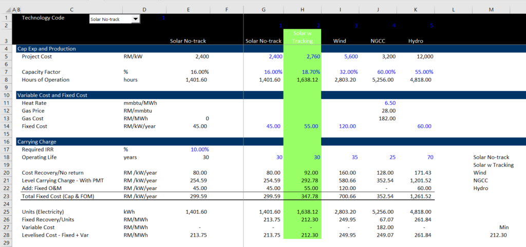
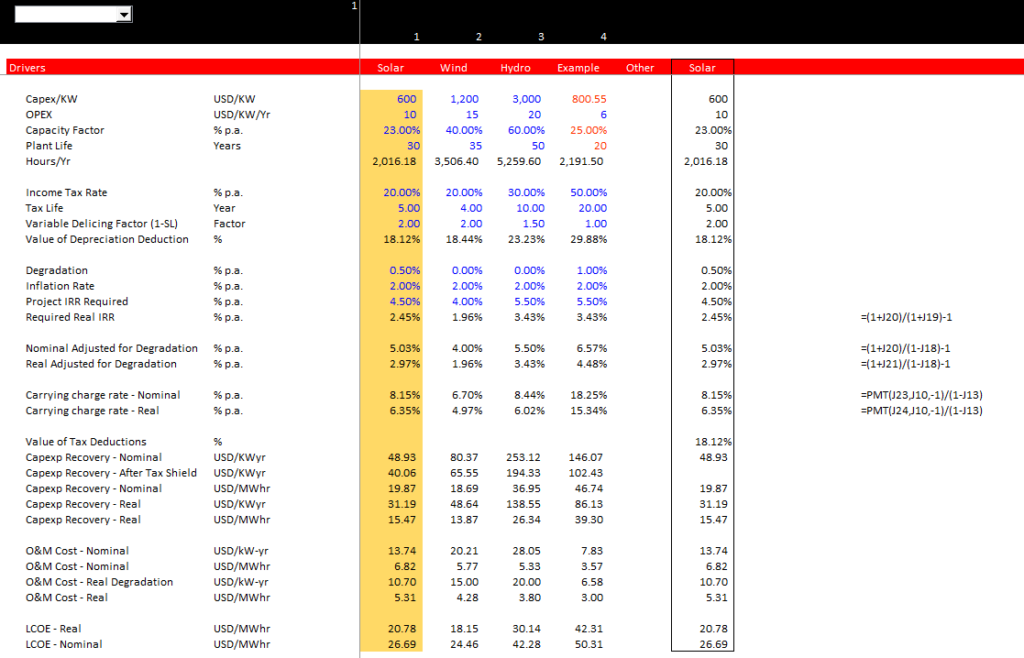
The screenshot below illustrates the starting point for computing levelised cost in a case without inflation, a case that I argue is an inappropriate case. To compute levelised cost in any situation, you need some drivers that include capital expenditures, operating costs, the lifetime of the project and some measure of the units sold. For a solar project, you can enter the capital expenditures per kW, the operating costs per kW-year, the lifetime and the capacity factor.
In this case the levelization — the word that is the foundation for levelized cost — can be accomplished with the PMT function that levelised payments over time. It is an absolutely essential function in excel that takes a single number and produces an equal payment that produces the net present value over a defined period as long as you give the formula a time period and also a discount rate. The payment formula is computed using the number one and the real discount rate in the above screenshot. As the lifetime of each project is different, the carrying charge rate is different for the four projects. The carrying charge rate is multiplied by the cost to produce the required carrying charges:
Carrying charge/kW-year = Capital Expenditure/kW x Carrying Charge Rate
With this the carrying charge, you can compute the carrying charge per unit. Then, assuming the O&M expense does not inflate — a very bad assumption — you can compute the levelised cost per unit using the following formula:
Hours Operated = 8766 x Capacity Factor
Carrying Charge/MWH = Carrying Charge/kW-year / Hours x 1,000
O&M/MWH = O&M/kW-year/ Hours x 1,000
Levelised Cost/MWH = Carrying Charge/MWH + O&M/MWH
Once the levelised cost is computed, alternative calculations of the LCOE can be demonstrates. These calculations are extremely simple in the case with flat units sold and with flat prices. But I begin the section by demonstrating the alternative formulas. To illustrate the other methods, I first make a very simple model. I have input the LCOE as the price and not put in any inflation, taxes, degradation or debt financing. Note that this model with a simple switch for the life produces and IRR that is the input target IRR. You can look at the details and see that the price is the same as the table above.
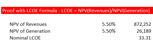
With this model you can compute use the classic formula for LCOE shown below. The results of this formula which produce the nominal levelised cost of electricity is shown below the formula in the screenshot. Note that the discount rate used for the NPV is shown next to the calculation. In this case the discount rate does not make a difference.
LCOE Nominal =
NPV(Nominal Rate, Revenues)/NPV(Nominal Rate, Units of Generation)
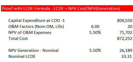
The third method involves using the NPV of costs rather than the NPV of revenues. If you use the same discount rate with the O&M costs — you can compute this with the PV formula in excel (not the NPV formula). Note that the total cost including the Capital Expenditure Cost plus the present value of the O&M cost over the life of the plant amount to the same value as the revenues.
LCOE Nominal = NPV(Nominal Rate, Costs)/NPV(Nominal Rate, Units of Generation)
The fourth method to compute the LCOE is a method where you compute what levelised cost really is — that is you levelise the price using a weighted average calculation. The weighting of the price so that it is not a simple weighted average price is driven by two things in the weighting. The first weighting factor is the amount of the generation. The second weighting factor is the discount rate where the amount of generation applied to the price is lower in future years. The weighted average calculation is shown in the screenshot below.