This page I addresses time series analysis and how to use Monte Carlo simulation to demonstrate various factors. Monte Carlo simulation can be used to demonstrate and prove some concepts in time series analysis including the increasing variance over time when there is no mean reversion, the concept of using continual growth versus discrete growth and how mean reversion can be derived using Monte Carlo Simulation. I include a lot of discussion of how to create Monte Carlo simulation in excel. I initially wrote this page when I was more enamoured with statisticians and proving every little thing in statistics book. I am revising the page to be somewhat more practical. Subjects on this page include:
- I begin with a non-mean reverting series and show how you can verify volatility measures and the increase in standard deviation of the rate of return over time by using Monte Carlo simulation. (You can compute the variance for a single simulation using the VAR.S function.)
- As volatility is the standard deviation of the rate of change or the growth rate or the rate of return, the increase in variance leads to the formula that volatility can be adjusted by the square root of time. For example, if you are computing the volatility for a month and you want the volatility for a year, you can use the formula:
-
- Annual volatility = Monthly Volatility x 12^.5.
- More formally, you could write
- Standard Deviation(Annual Rate of Change) = Standard Deviation(Monthly) x 12^.5
- To evaluate the increase in variance with long time periods (again without mean reversion), you can use the EXP function and assume continual growth rather than discrete growth in distributions as shown below:
- Continual Rate of Change = LN(Current Price/Prior Price)
- Please don’t worry, this is not fancy math, it is just used to prove the idea of increasing variance over time with non-mean reverting series.
- A second issue with Monte Carlo simulaton is getting things to work fast and creating efficient macros. Unlike the simple simulations of in the initial page, I show how to make a more interesting and much faster and more flexible simulation with some macros. This follows the idea that if you are making multiple calculations it is much faster to do them in a macro or in a user defined function.
- With the fundamental case established, I illustrate the testing measures in volatility output (for example using population or sample variance) given the volatility input and demonstrate how to measure the change in standard deviation as time progresses with no mean reversion and with full mean reversion.
My philosophy in understanding time series is to demonstrate how the statistics really work by using Monte Carlo proofs. These kinds of proofs are perhaps a more useful application of Monte Carlo simulation than attempting to put Monte Carlo simulation into your financial models. At the end you can hopefully think about mean reversion and volatility and use the notions in a conceptual way to derive debt terms and risk analysis.
You can download the file below that includes simulations of brownian motion and mean reversion. This file includes discrete and continuous equations with random (stochastic) variation. It also includes VBA code that you can use to make more efficient simulations. Some of the conclusions from this simulation analysis include:
- Use the sample variance and then take the square root of the sample variance in computing the volatility generated from the simulation. This will match the volatilty input.
- You could compute the volatilty factor as P1 x volatility x Normal Inverse. Alternatively, you could use EXP function which is like (1+Volatility Factor). The simulation demonstrates that it is better to use the EXP function.
- When there are more data in the series, e.g. modelling daily instead of annually, you will get a better value.
.
Step by Step:
- Make simulation with EXP(Vol x Rand) or with 1 + Vol x Rand.
- Compute the Variance — not the standard deviation — of each simulation using the VAR.S function.
- Compute the average (or the median) of each of the Variance statistics that comes from each simulation
- Once the average variance is computed for each simulation, compute the average and then after you compute the average, take the square root to compute the standard deviation which is the volatility
- Compare the computed volatilty with the input volatility and it should be similar as demonstrated in the screenshot below.
The conclusion is that you should use the variance with the sample and not the population
The second conclusion is that you should use the
.
.
.
Excel File with Analysis of Monte Carlo Simulation Using Alternative Mean Reversion Parameters
.
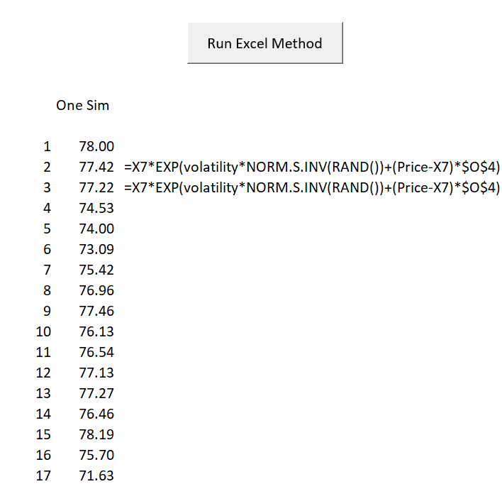
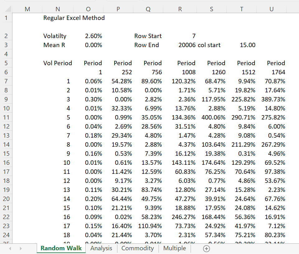
Simulating with Excel RAND
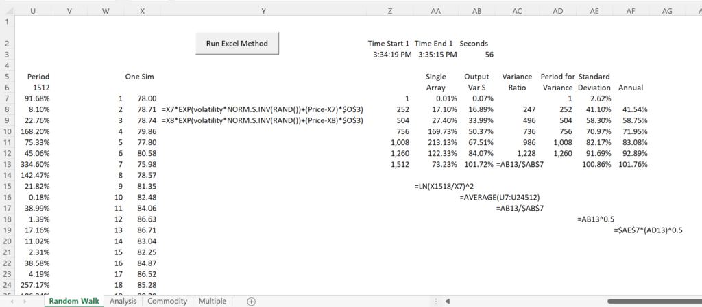
The code below illustrates how you can make a simulation directly in excel or you can write the code for equations in VBA. The direct excel is easier and even faster, but the VBA is more accurate, apparently because of different random numbers. The simple method is illustrated by the screenshot and the code below.
The VBA code uses this one_simulation column and retains the variance. Then the variance is used to assign to an array. Each different variance for different length periods is retained. The time start and the time end is also retained. The VAR_P is written for each simulation and then this result is put into the CELLS output.
.
Sub simulate_raw()

Range("time_start_1") = Time
col = Range("col_start")

Application.ScreenUpdating = False
current_status = Application.Calculation
Application.Calculation = xlCalculationManual

For Row = Range("row_start") To Range("row_end")

    Range("one_simulation").Calculate

'    ActiveSheet.Calculate

    Range("varp_array").Calculate

    Cells(Row, col) = Range("varp_array").Cells(1, 1)
    Cells(Row, col + 1) = Range("varp_array").Cells(2, 1)
    Cells(Row, col + 2) = Range("varp_array").Cells(3, 1)
    Cells(Row, col + 3) = Range("varp_array").Cells(4, 1)
    Cells(Row, col + 4) = Range("varp_array").Cells(5, 1)
    Cells(Row, col + 5) = Range("varp_array").Cells(6, 1)
    Cells(Row, col + 6) = Range("varp_array").Cells(7, 1)

Next Row

Range("time_end_1") = Time

Application.Calculation = current_status

End Sub
The individual cells that are written are illustrated in the screenshot below. The rows are written with each simulation as shown in the code above. Note that results are all over the place.
.
The final results are illustrated below.
Simulating Random Walk with VBA and RND
The VBA code and screenshots below illustrate the same number of simulations using VBA code. In this code, the time series equation is part of the code rather than in excel. The process takes more time (I don’t know why). But it consistently produces more accurate results. The more accurate results are illustrated by the variance relative to the first period which should equal the number of periods.
The VBA code that also prints out individual scenarios is shown below. The code is longer with formulas for the time series. When you output, you need a row and a column. You can put the entire output in a different sheet and then use this for financial model scenarios.
Sub math_simulate_multiple()

Dim sim_num, number_in_series, mod_test As Single

sim_num = InputBox(" Enter the Number of Simulations ", , 2000)
number_in_series = InputBox(" Enter the Number in Series ", , 1800)

'Volodymyr Zelensky

Dim price_sim(), average_sim(), pct_change() As Variant
Dim pct_change_252(), pct_change_504(), pct_change_756(), pct_change_1008() As Variant
Dim pct_change_1260(), pct_change_1512(), pct_change_1764() As Variant
Dim avg_output(8, 1) As Double

ReDim price_sim(number_in_series, sim_num), average_sim(number_in_series, 1)
ReDim pct_change(sim_num)
ReDim pct_change_252(sim_num), pct_change_504(sim_num), pct_change_756(sim_num), pct_change_1008(sim_num)
ReDim pct_change_1260(sim_num), pct_change_1512(sim_num), pct_change_1764(sim_num)

sheet_name = "Multiple"
range_name = "=" & sheet_name & "!R" & 10 & "C4:R" & 10 + number_in_series - 1 & "C" & 4 + sim_num

MsgBox range_name

On Error Resume Next
ActiveWorkbook.Names("output").Delete
ActiveWorkbook.Names.Add Name:="output", RefersToR1C1:=range_name

Range("time_start") = Time

Range("sim_num") = sim_num
Range("number_in_series") = number_in_series

price_sim(1, 1) = Range("price").Value
mean_price = Range("price").Value
volatility = Range("volatility").Value
mean_reversion = Range("mean_reversion").Value

Range("mc_output").Clear

'    MsgBox " Mean Reversion " & mean_reversion & " Price Sim " & price_sim(1) & " Volatility " & volatility

 For simulation = 1 To sim_num

    price_sim(1, simulation) = Range("price").Value

    mod_test = 100
    mod_test = 100 Mod simulaton
    mod_test = simulation Mod 100

    If mod_test = 0 Then

         UserForm1.Label1 = " Simulation " & simulation & " Volatilty " & volatility & " Mean Reversion " & mean_reversion
'        UserForm2.Label1 = " Simulation " & simulation
         UserForm1.Label2 = " Number of Simulations " & sim_num & " Length of Series " & number_in_series

     DoEvents

    End If

    For Row = 2 To number_in_series

        rand_num = Rnd()

        On Error Resume Next
        Norm_S_Dist = WorksheetFunction.Norm_S_Inv(rand_num)

'        price_sim(Row, 1) = price_sim(Row - 1, simulation) _
'                       + (mean_price - price_sim(Row - 1, simulation)) * mean_reversion _
'                       + price_sim(Row - 1, simulation) * volatility * Norm_S_Dist


        price_sim(Row, simulation) = price_sim(Row - 1, simulation) * Exp(volatility * Norm_S_Dist) + _
                        (mean_price - price_sim(Row - 1, simulation)) * mean_reversion _

'        pct_change(Row) = WorksheetFunction.Ln(price_sim(Row, 1) / price_sim(Row - 1, 1))

        If Row = 2 Then pct_change(simulation) = WorksheetFunction.Ln(price_sim(Row, simulation) / price_sim(Row - 1, simulation)) ^ 2
        If Row = 253 Then pct_change_252(simulation) = WorksheetFunction.Ln(price_sim(Row, simulation) / price_sim(Row - 252, simulation)) ^ 2
        If Row = 505 Then pct_change_504(simulation) = WorksheetFunction.Ln(price_sim(Row, simulation) / price_sim(Row - 504, simulation)) ^ 2
        If Row = 757 Then pct_change_756(simulation) = WorksheetFunction.Ln(price_sim(Row, simulation) / price_sim(Row - 756, simulation)) ^ 2
        If Row = 1009 Then pct_change_1008(simulation) = WorksheetFunction.Ln(price_sim(Row, simulation) / price_sim(Row - 1008, simulation)) ^ 2
        If Row = 1261 Then pct_change_1260(simulation) = WorksheetFunction.Ln(price_sim(Row, simulation) / price_sim(Row - 1260, simulation)) ^ 2
        If Row = 1513 Then pct_change_1512(simulation) = WorksheetFunction.Ln(price_sim(Row, simulation) / price_sim(Row - 1512, simulation)) ^ 2
        If Row = 1765 Then pct_change_1764(simulation) = WorksheetFunction.Ln(price_sim(Row, simulation) / price_sim(Row - 1764, simulation)) ^ 2

    Next Row

     If mod_test = 0 Then                   ' Go between the two forms
         UserForm1.Show vbModeless
 '        Unload UserForm2
     End If

     If simulation Mod 200 = 0 Then                   ' Go between the two forms
'         UserForm2.Show vbModeless
'         Unload UserForm1
      End If

    Next simulation


'    MsgBox " Pct chg 1 " & pct_change(1)

'   average_1 = WorksheetFunction.Average(pct_change)
'   average_2 = WorksheetFunction.Average(pct_change_252)
'   average_3 = WorksheetFunction.Average(pct_change_504)
'   average_4 = WorksheetFunction.Average(pct_change_756)
'   average_5 = WorksheetFunction.Average(pct_change_1008)
'   average_6 = WorksheetFunction.Average(pct_change_1260)
'   average_7 = WorksheetFunction.Average(pct_change_1512)
'   average_8 = WorksheetFunction.Average(pct_change_1764)

   avg_output(1, 1) = WorksheetFunction.Average(pct_change)
   avg_output(2, 1) = WorksheetFunction.Average(pct_change_252)
   avg_output(3, 1) = WorksheetFunction.Average(pct_change_504)
   avg_output(4, 1) = WorksheetFunction.Average(pct_change_756)
   avg_output(5, 1) = WorksheetFunction.Average(pct_change_1008)
   avg_output(6, 1) = WorksheetFunction.Average(pct_change_1260)
   avg_output(7, 1) = WorksheetFunction.Average(pct_change_1512)
   avg_output(8, 1) = WorksheetFunction.Average(pct_change_1764)

   Range("avg_output") = avg_output

   Range("time_end") = Time

    ActiveSheet.Calculate

   Unload UserForm1
'   Unload UserForm2

   Range("output") = price_sim

Exit Sub

 For Row = 1 To number_in_series
     For simulation = 1 To sim_number

        average_sim(Row, 1) = average_sim(Row, 1) + price_sim(Row, simulation)

     Next simulation

     average_sim(Row, 1) = average_sim(Row, 1) / 100

 Next Row

    Range("mc_output") = average_sim

 Exit Sub

For Row = 1 To 50
    Range("mc_output").Cells(Row, 1).Value = price_sim(Row)
Next Row

End Sub
The VBA code with some of the concepts is illustrated below. I make a flexible range name. I should do all of the math inside the VBA code, but I have just been doing this recently. Note how the range name is flexible so that you can use different numbers of simulations.
Sub simulate()
On Error Resume Next
Range("output").ClearContents ' Clear out the prior scenario
'
' Now make a range name from the number of scenarios and the number of outputs
'
sheet_name = ActiveSheet.Name
range_name = "=" & sheet_name & "!R" & Range("row_start") & "C4:R" & Range("row_start") + Range("simulations") & "C12"

ActiveWorkbook.Names("output").Delete
ActiveWorkbook.Names.Add Name:="output", RefersToR1C1:=range_name

Application.ScreenUpdating = False

Dim output_range() As Variant ' Note that you should make an array without any dimension
ReDim output_range(Range("simulations"), 9) ' Use the input to put in the dimensions of the output

For I = 0 To Range("simulations")
     Range("volatility_output").Calculate ' This is to make a very little calculation like pressing the F9

     output_range(I, 1) = Range("vol_1") ' Now put the outputs into the arry
       output_range(I, 2) = Range("vol_1a")
       output_range(I, 3) = Range("vol_2")
       output_range(I, 4) = Range("vol_2a")
       output_range(I, 5) = Range("vol_3")
       output_range(I, 6) = Range("vol_3a")
       output_range(I, 7) = Range("vol_4")
       output_range(I, 8) = Range("vol_4a")
Next I

Range("output").Value = output_range
End Sub
Setting Up Brownian Motion and Mean Reverting Time Series
I will use some time series equations to illustrate the various points relating to Brownian motion time series and mean reverting time series. Begin by understanding that the measured volatility is the standard deviation of the rate of return or the rate of change in price. When I first started applying Monte Carlo simulation I did it in a blind and mechanical way by just copying the method where you first compute the percent change using the formula change = Pt/Pt-1 – 1 or percent change = LN(Pt/Pt-1). The first formula assumes that the change occurs at the end of the period and the second assumes that changes occur at infinitely small increments over the period. The standard deviation of the rate of return is the volatility. If the time increments are annual, the volatility can be expressed as annual volatility. In the screenshot below, I assume that the annual volatility is 10% and the expected return is 4%. If you assume the returns are normally distributed (not the absolute prices) then there should be a 68% chance that the return will be between one standard deviation above the mean and one standard deviation below the mean. If you are like me and you need to remind yourself of this, you can compute the cumulative normal distribution for a series of returns as shown in the screenshot below. At the end of the day, the volatility gives you probabilities of returns above or below the expected return. In the case below, there is a 68% chance that the return will be between 14% and -6%. You can hopefully see like me that this only works if the returns (not the stock prices) come from a normal distribution.
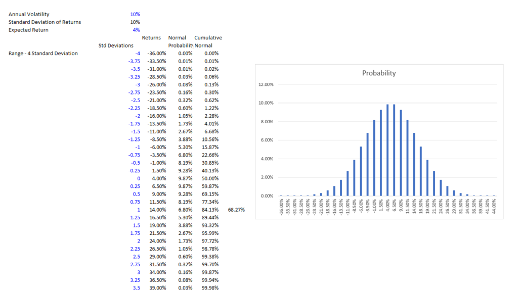
To allow the return to change, you can apply a volatility factor to the return. This can be done as shown below by using the RAND() function in excel and then applying a distribution assumptions to the random number. For this case I assume that numbers come from a normal distribution (I will discuss this later a lot.) To apply the normal distribution, I use the inverse of the normal distribution the produces a value instead of a probability. The inverse of the normal distribution can be used with a mean of zero and a standard deviation of 1.0. When you put a standard deviation into the standard normal distribution, you will get a probability between zero and 1. Conversely, you can use the NORMSINV function to give you a standard normal value with a mean of zero and a standard deviation of 1.0 by inputting the RAND function using NORMSINV(RAND()). This is illustrated below.
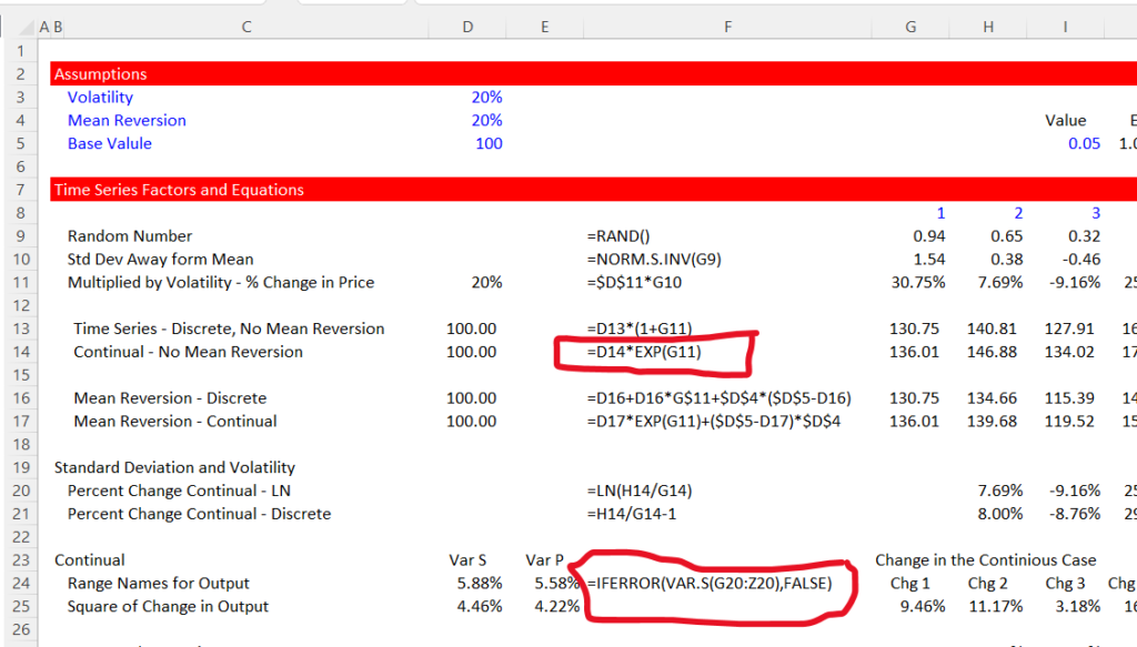
I use discrete and continuous time series equations in my Monte Carlo simulation tests. The time series equations with stochastic variation are illustrated in the screenshot below. As shown, I start only with a volatility statistic and a mean reversion statistic. I use a discrete time series where the change is all assumed to occur at the end of the period. When you use something like Price t = Price t – 1 * (1 + return), you are assuming that the return you input occurs at the end of the period. If you want to assume that the return occurs at tiny increments or incrementally over the time period, you can use the formula Price t = Price t – t x exp(return).
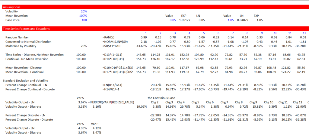
In this sheet, when you press the F9 key in excel you will get a different scenario. My idea with Monte Carlo simulation is to test various things about a mean reverting series and a non-mean reverting time series with this simple Model
More Efficient VBA Code for Monte Carlo Simulation
The first Monte Carlo simulation I made was to test whether the volatility that you input is the same as the volatility that results from the scenarios. To do this you can make a whole bunch of simulations and than compute the average or median volatility across the different scenarios. I don’t know whether to use the population standard deviation or should I compute the variance for the different scenarios and then take the square root. Further, should I compute the volatility with the LN function on the continuous time series and the discrete percent change with the discrete function. I could try to look around my old statistics books for this, but I think it is better to prove things with a Monte Carlo simulation where you can compute the percent change (the growth rate) from period to period and then compute the standard deviation or the variance of the growth rate.
When running a simulation to test things, I want to be able to run a whole lot of simulations but I don’t want to sit around and wait for hours. If I can compute tens of thousands of simulations then I can run it again and test if I get the same answers. To make a more efficient simulation in VBA you can try a couple of things. The first is to use the APPLICATION.SCREENUPDATING = FALSE. Then you can get a little more complicated and save the scenarios into an array rather than writing each scenario out separately. To do this you can make a flexible array as shown in the code below where you could make an array named output with DIM Output() as variant. Then you can use the REDIM statement with the number of simulations and output variables that you want.
Sub simulate()
On Error Resume Next
Range("output").ClearContents ' Clear out the prior scenario
'
' Now make a range name from the number of scenarios and the number of outputs
'
sheet_name = ActiveSheet.Name

range_name = "=" & sheet_name & "!R" & Range("row_start") & "C4:R" & Range("row_start") + Range("simulations") & "C12"

ActiveWorkbook.Names("output").Delete ActiveWorkbook.Names.Add

Name:="output", RefersToR1C1:=range_name

Application.ScreenUpdating = False

Dim output_range() As Variant
' Note that you should make an array without any dimension

ReDim output_range(Range("simulations"), 9)
' Use the input to put in the dimensions of the output

For I = 0 To Range("simulations")
Range("volatility_output").Calculate ' This is to make a very little calculation like pressing the F9

output_range(I, 1) = Range("vol_1") ' Now put the outputs into the array
output_range(I, 2) = Range("vol_1a")
output_range(I, 3) = Range("vol_2")
output_range(I, 4) = Range("vol_2a")
output_range(I, 5) = Range("vol_3")
output_range(I, 6) = Range("vol_3a")
output_range(I, 7) = Range("vol_4")
output_range(I, 8) = Range("vol_4a")
Next I
Range("output").Value = output_range
End Sub
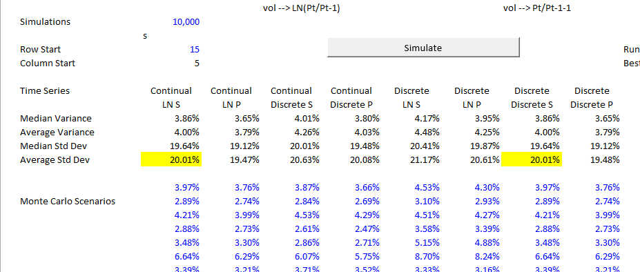
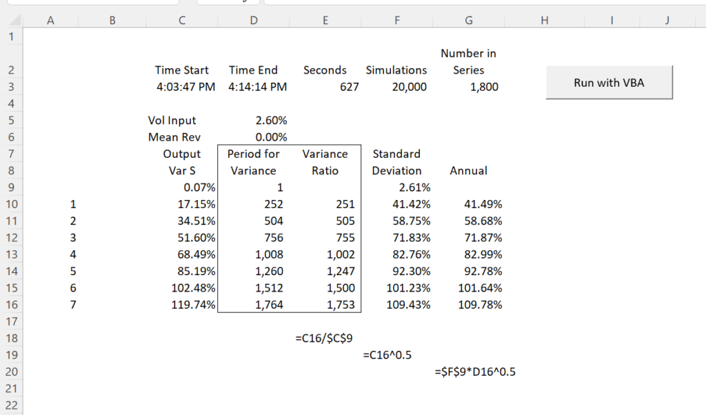
The screenshot below demonstrates a simulation with 40,000 draws that only takes seconds. I have tried a couple of things in computing the volatility output where the input volatility was 20%. As shown on the screenshot, the volatility output is 20% when you compute the growth rate as LN(price t/price t-1) and then take the variance. When you average all of the 40,000 scenarios and use the sample variance rather than the population variance, then the square root of the average variance is the same as the input volatility.
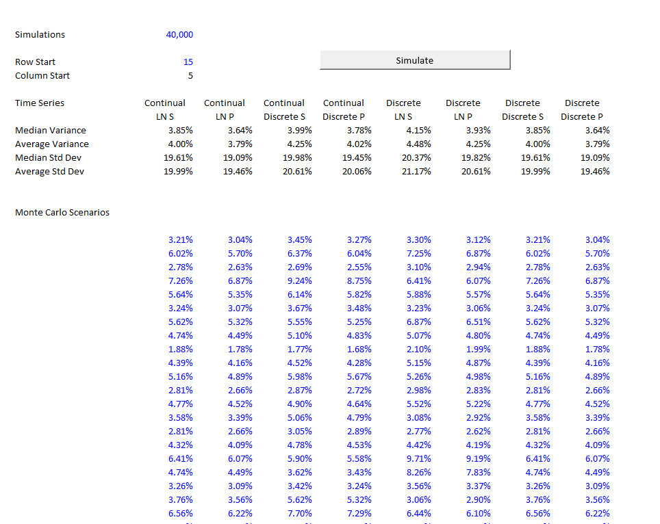
Note also that when you use a discrete distribution rather than the EXP function, the volatility output that gives you the same as the volatility input is the sample variance with the volatility computed from discrete growth rates. With this base, you can start looking at a lot of stuff. You can test whether the Black-Scholes model produces the same results with Monte Carlo simulation; you can test what happens when you use mean reversion; you can evaluate correlations; you can make equations with upper and lower boundaries to represent surplus and excess capacity and then evaluate whether your model is producing volatility results consistent with the observed historic volatility ….
Testing the Increase in Volatility Over Time in Brownian Motion
When you apply volatility in a model, I was told a long time ago that you should multiply the volatility (the standard deviation of growth or the standard deviation of return) by the square root of the number of periods per year to annualise the volatility:
Volatility = Standard Deviation of Returns x Square Root (Periods per Year)
For example, if you have monthly data, you can compute the standard deviation of returns on a month by month basis. Then, once you have the monthly volatility, you multiply the number by the square root of 12. This is the central idea I will use in evaluating whether the series is a mean reverting series. The idea that volatility increases over time in a non-mean reverting series is intuitive. The idea of a square root seem reasonable as volatility is a standard deviation. But for me it stops there. I could go to a statistics book and maybe find a proof of the formula. But that would be a real pain and I would probably not understand all of the math.
Instead of doing this, you can compute the growth rate from the initial period with either LN or with the discrete percent change for each of the different time periods. Then I bring the data labeled Chg_1, Chg_2 and Chg_3 … into the Monte Carlo simulation.
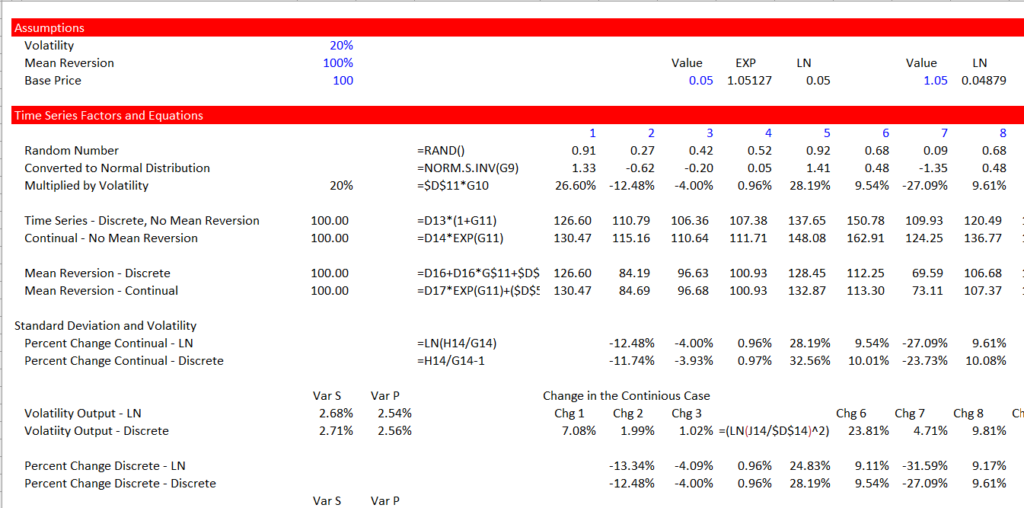
In the above screenshot I compute the change in the price relative to the initial price. As there is no trend in the price, the expected change in price over multiple scenarios is zero (you can test this with the Monte Carlo simulation). If you computed the percent change in price relative to the initial price you can compute the variance as the square of the percent change in price. You can then compute this change in price squared relative to the initial price for different periods. The variance should increase over time as a Brownian motion series keeps moving up or down and does not come back to the mean. Indeed, as discussed above, the standard deviation should of returns should increase with the square root of time. This means in the screenshot above, the standard deviation of the change in price for the second period should be the square root of 2 relative to the first period. I want to demonstrate this in a rigorous manner because I will use this idea to discuss mean reversion.
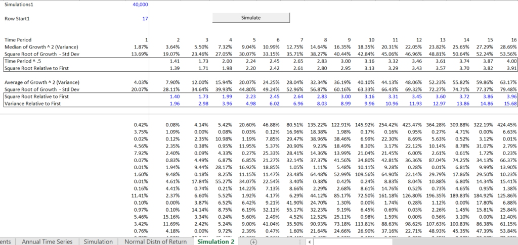
The screenshot below shows the results of the simulations using 40,000 simulations. The output of the 40,000 simulations is the square of the change in price relative to the first price — LN(Pt/Po)^2. After computing the variance, I compute the average variance and the median variance across the 40,000 simulations. This is shown in the screenshot below. Then I compute the standard deviation of the variance — both the average and the median. You can see that the variance increases each period as expected. Then, finally, I compute the standard deviation relative to the first period. I compare this to the standard deviation of 2, 3, 4 etc. Note that the increase in the standard deviation is just about the same as the square root of the period. The average for the first period is just about the same as the volatility. Then the second period standard deviation is 1.42 while the standard deviation of the 2 is 1.42. You can also see that in terms of variance, the variance increases in direct proportion to the the time period where the variance in the second period is just about double the variance of the first period.
This whole thing with Monte Carlo simulation is a really big deal to me. We now have a tool to evaluate what happens not only to the volatility output from our equations, but we also have a tool to test when we change mean reversion parameters or input lower or upper boundaries, what in theory should happen to the change in standard deviation over time.
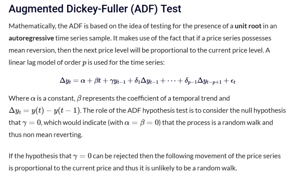
Testing for Mean Reversion
The manner in which statistical tests are constructed for mean reversion illustrates the problem for me. When you try to test for the presence of mean reversion or better yet, derive the mean reversion parameter, the tests are not very useful for me at all. The excerpt below illustrates a test that apparently is what I use to test for autocorrelation in a series. I suggest a much more intuitive way to derive mean reversion is to use the above principle that without mean reversion the standard deviation increases over time.