This page demonstrates how to convert a normal corporate model into an acquisition model after you have completed the standalone corporate model. Conversion of the model into an acquisition model for M&A analysis involves inserting a page with acquisition assumptions as well as a sources and uses of funds analysis, a goodwill analysis and a pro-forma balance sheet. Acquisition assumptions include the premium paid above the current stock price, the manner in which the acquisition is financed; the amount of synergies and transaction costs from the acquisition. These steps are described in the discussion below, continuing with the case that has been used to explain the other steps in corporate modelling. In the exercise, you walk through transaction assumptions, then construct a sources and uses of funds and pro-form analysis. After setting-up the transaction, you can see how a cash flow waterfall with multiple debt tranches works in the context of an acquisition analysis. You can download the files attached to the buttons below and work either with the file with the completed analysis or the file that I made which has blanks so that you can work through some of the key acquisition modelling equations. When you open the model, go to the pages name “Acquisition Transaction” and the page named “Acquisition Model”.
Assumptions and Transaction Page
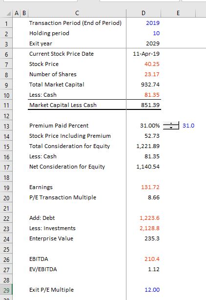
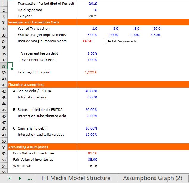
After you have completed your standalone model you can begin working on the transaction assumptions. You can insert a new page and then begin by entering the date of the transaction. This date should correspond to a date in the standalone model so that you can use the LOOKUP function a lot. The screenshot below illustrates how the LOOKUP function is used first to collect information on the number of shares. Once you have the dates and the shares defined you can define the purchase price and equity consideration in various different ways. In the screenshot below, I define the premium as a percent of equity and then the equity consideration can also be defined. As the enterprise to equity bridge has been defined in the standalone model, the total enterprise value can be defined. Then, you can also put in the EBITDA and the net income to compute transaction multiples. The final assumption in this part of the Transaction inputs is the exit multiple that you will assume when you sell the company. The exit multiple is necessary computing the IRR on the transaction. After you have entered the purchase price assumptions you can put in some data on the expected synergies and the fees. I have entered the synergies as a margin on the EBITDA and put in staggered years so that you can practice using the INTERPOLATE function. The next section of the transaction assumptions is where you should enter data about how the transaction will be financed and include assumptions about whether existing debt will be assumed or re-paid. The final part of the transaction assumptions involves the accounting assumptions. I have just entered a couple of items here to illustrate how the accounting works in the pro-forma balance sheet. To re-emphasize, the LOOKUP function can be used a whole lot here to gather the appropriate data.
Sources and Uses of Funds
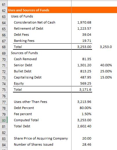
The next step in constructing an acquisition model is to create a sources and uses of funds statement. You can begin with the uses of funds that include the consideration, the retirement of debt and the fees. The sources of funds consist of the different debt issues and the equity that must be raised for the transaction (this equity could come from cash contributions, a share exchange or even an earn out from existing shareholders. This is the major calculation in the sources and uses of funds statement and it is a simple subtraction. If you have the share price of the acquiring company, you can also compute the number of shares issued that will ultimately be used in computing accretion or dilution. Finally, as the debt in this model is assumed to be from the debt to capital ratios, a little circular reference problem arises with the total uses. This can be resolved with a bit of algebra as shown in the equations below. Note that in the equations, the total represents the total uses of funds that include debt fees. The screenshot below the equations illustrates how you can apply this bit of algebra and the layout of the sources and uses of funds.
- total = other + debt fees
- debt fees = total debt * percent
- total = other + total debt * fee percent
- total debt = total * debt percent
- total = other + total * debt percent * fee percent
- total – total * debt percent * fee percent = other
- total * (1-debt percent * fee percent) = other
- total = other /(1-debt percent * fee percent)
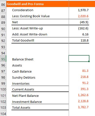
Goodwill and Pro-Forma Balance Sheet
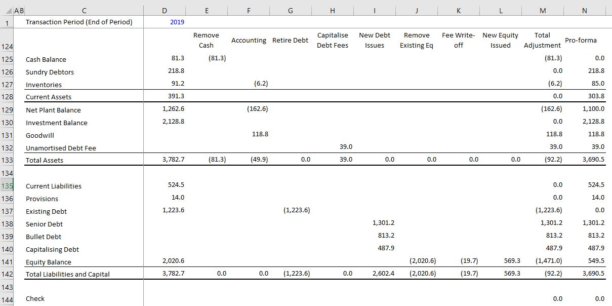
For computing the pro-forma balance sheet, you first should compute the goodwill. The formula in a model to compute goodwill can be derived from the total equity consideration less the existing book value. In this case, unless the premium is really big, the goodwill will be negative. So, to illustrate the accounting, I put in a really big premium. Note that if the goodwill is negative, you are supposed to work through the balance sheet and write-down assets to their fair value. Once you have computed the goodwill, you can go begin to put the balance sheet together. To get in the existing balance you can use the LOOKUP and take the titles from the balance sheet. Then you can put in a cleaned up balance sheet that has the accounts that you want. When you set-up the balance sheet, there are a couple of rules and practices I suggest. First, set-up the balance sheet format with goodwill, unamortised debt fees and put in the new debt issues. This will provide opening balances for the period by period acquisition model. Next, when you start to put in adjustments to the balance sheet from the transaction, put the different items in separate columns. This makes the model much more transparent. You can then create sums at the bottom and across the adjustments. Finally, understand that every single adjustment item comes from either the sources and uses statement or the goodwill section. The pro-forma sheet with our example is illustrated in the screenshot below.
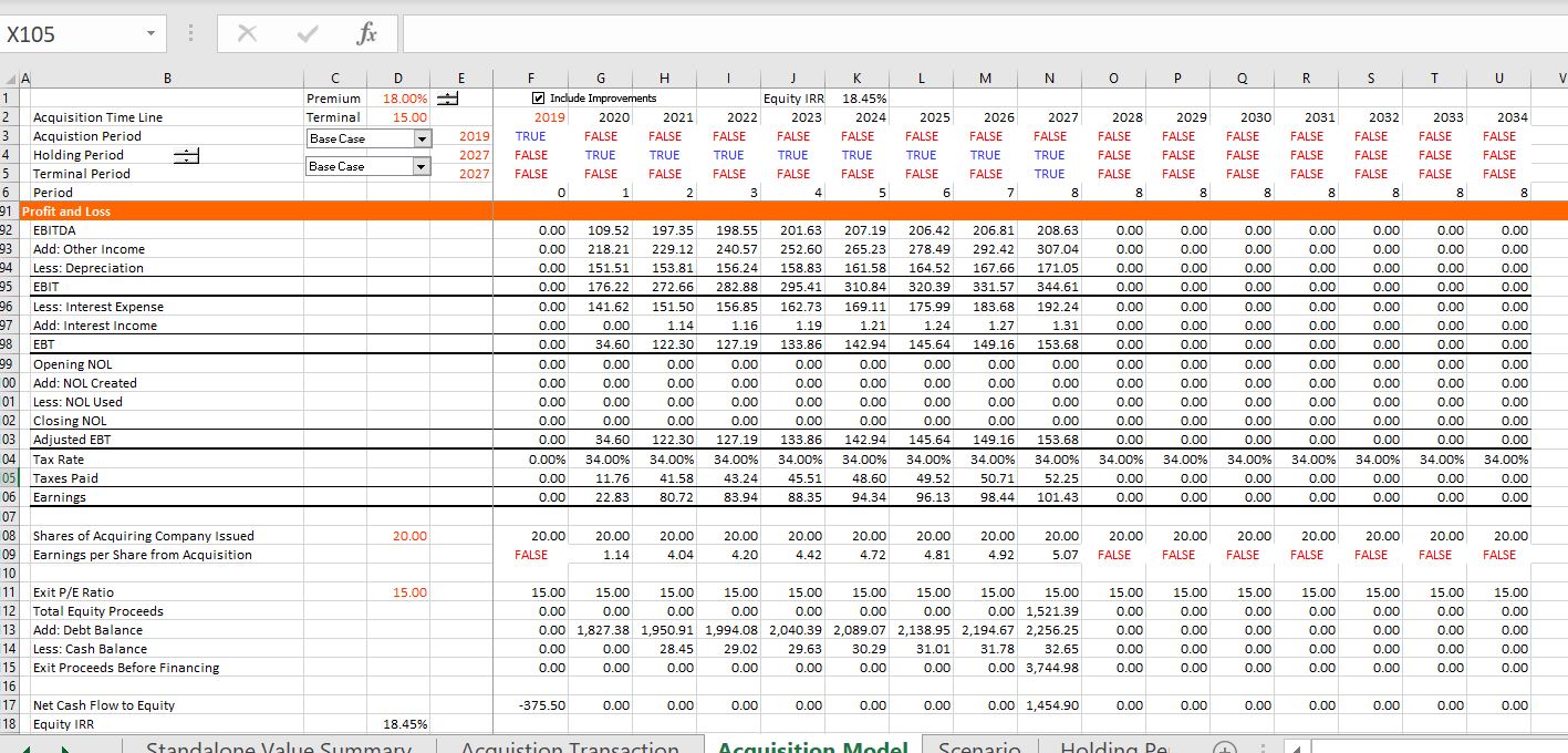
Financial Model of the Acquisition
The first step in the model, like in any model is to create a time line. As with the valuation section the time line should also include a switch for the holding period and the terminal period. This is done with the normal TRUE/FALSE switches and I have put a spinner box next to the holding period so that you can evaluate the effect of different sale dates. With the time line defined, you can put in the pro-forma balance sheet that you computed in the last step which is analogous to the historic balance sheet in the regular old stand alone model. After that, you should collect all of the stuff from the pre-tax and post-tax part of the model for EBITDA, Capital expenditures, depreciation and so forth using the LOOKUP function — you don’t have to do the hard part of the modelling which is deriving the assumptions. (I am assuming this is a tax free exchange of shares so not making an adjustment to the tax depreciation). The only exception to simply bringing in data is the synergy analysis which can affect the operating expenses, the revenues and the capital expenditures which is shown in the screenshot below along with the time line. Much of the model then has the same structure as any corporate model, with free cash flow first (the transferred variables), then setting-up the financing, then working through the financial statements and finishing up with the balance sheet. The balance sheet calculations maybe a little different in an acquisition model as the balances may be derived from the pro-forma starting balance sheet and the cash flow changes (for example, you may consolidate the working capital and adjust the plant balance for the sale of assets). I discuss how to model financing of the transaction and the cash flow waterfall in the next section. As much of this is the same as the structure of a normal old financial model, I do not repeat the boring discussion here. You can open the file above and look at the structure.
Financing Structure and Cash Flow Waterfall
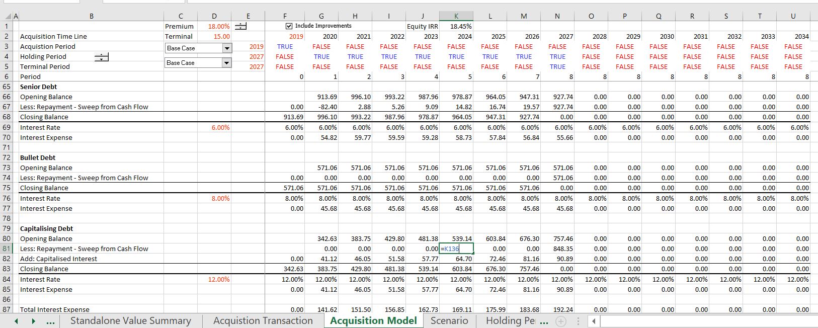
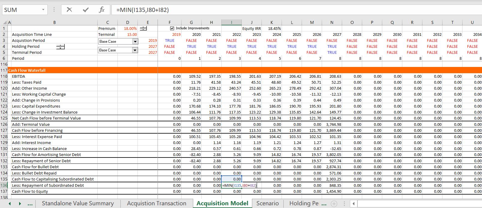
As in any model there should be a separate section where you work through the financial instruments which in this case are three tranches of debt. I have put the balances of the debt into the model directly from the cash flow statement and assumed that each of the three debt facilities is repaid from a cash flow sweep. If the debt is paid from a cash sweep or the debt is defaulted debt, or an escrow account is used to make up cash flow short-falls, then you should find the repayment not from some complicated calculation in the debt balance, but instead, directly from the cash flow statement. This means that you put in financing balances and refer to the cash flow. The process is illustrated in the two screenshots below. The first screenshot below this paragraph shows how you can lay out the three debt issues with opening and closing balances. I have assumed that the third facility is capatalising debt which means that the debt balance increases for interest that is not paid. In terms of the cash flow waterfall, I have assumed that the senior debt receives the cash first but that the interest on the bullet debt is paid. This is illustrated on the second screenshot that shows and example of the cash flow waterfall layout. The capitalised debt only receives cash flow after the first facilities are paid and may have to be paid from the terminal proceeds. The manner in which you can set-up the cash flow waterfall that determines how much debt is re-paid and which debt tranche has the most risk. You should set-up the cash flow waterfall in the same order as the cash is used and then connect the repayments of the different facilities to the debt balances shown in the first screenshot. When you create equations in the cash flow waterfall, the key is to use the MIN function with cash flow from the sub-total line above and the opening balance of the debt. I have discussed this use of the MIN function a lot elsewhere and this example is pretty simple with perhaps a small complication for the capitalising debt issue. In this case, the MIN function should include the capitalised interest which increases the balance of the debt. I hope it is apparent from looking at the screenshot that to use the MIN function with the opening balance, you should set-up a lot of sub-total accounts as shown in the second screenshot.
Cash Flow and Valuation in Acquisition
Once you have the cash flow and the income statement completed, you can make different assessments of the value of the transaction. A primary statistic is the IRR earned on equity. To make this calculation you go to the bottom of the cash flow statement with the net cash flow to equity. You then add the amount of equity contributed by equity holders to get the initial negative cash flow. This equity contribution number comes from the sources and uses of funds that was derived on the transaction assumptions page. The calculation of equity IRR on the transaction is illustrated at the bottom of screenshot below. The screenshot also shows how you can gauge the effect of the transaction on the earnings per share of the acquiring company. To make this calculation, you should first determine how many new shares of the acquiring company are directly or indirectly issued for the transaction. This calculation is shown in the sources and uses of funds statement above where the equity issue is divided by the share price of the acquiring company. With the shares defined, the effect of the acquisition on the earnings per share of the acquiring company is the earnings divided by the new shares. This amount of shares should be compared with the forecasts of earnings per share on a standalone basis. The screenshot below also shows calculation of the exit value. This exist value could be computed using an EV/EBITDA ratio or a P/E ratio or a Price to Book ratio. I have used the P/E ratio and multiplied the P/E exit value by the projected earnings. As the P/E ratio only measures equity value and the debt proceeds and cash payments are below the terminal proceeds and come out of the terminal proceeds, these items must be added to or subtracted from the equity proceeds.