This page describes debt sculpting in project finance when there are multiple debt issues all of which are sculpted, but some have different interest rates and tenures. In this case of multiple different debt issues, allocation of sculpted debt repayment to different issues with different interest rates and different debt tenures, the calculations are more complex because the size of the debt is driven by the cash flow and also by the given fixed amount debt or percent of total debt. An example of this type of situation with multiple debt issues is when there is an issue from a development finance institution as well as an issue from a private bank. For example, the commercial bank may often be sculpted in the same manner as the development finance institution, but have a short tenure. To sculpt with multiple issues, you can use the following few concepts. First, compute the overall debt IRR using the aggregate debt service and the aggregate debt issues (you don’t know this until you are finished). Second, split the debt issues between the capture debt issue (the longest tenure) and the other non-capture debt issues. For the non-capture debt issues, use the LLCR method to compute sculpting where you compute the PV of CFADS and divide by the size of the individual issue.
.
Modelling Multiple Debt Issues All with Sculpted Repayment with Different Tenures and Different Interest Rates Using Capture and Non-Capture Issues
This section moves from fairly basic issues to a difficult issue where you are not given repayment on the non-sculpted debt issues, but you have to compute sculpted repayment on many debt issues. The mechanics of computing multiple sculpting is more difficult than where you have one sculpted debt issue and one non-sculpted issue as in the case of the balloon payment. As shown above, the modelling of sculpting is not all that difficult where only one of the debt issues is sculpted. You can use the formula to derive the sculpting by using the following formula:
Sculpted Issue DS = CFADS/DSCR – Other DS
If other debt issues are sculpted, this formula does not work in a simple manner. In this section I explain how you can compute sculpted debt repayments and debt service when you have multiple debt issues with different terms (tenures and interest rates). I have put together a file that includes issues of calculating debt service for multiple debt issues in the file below.
.
.
.
.
.
Capture Debt Issue and Steps to Compute Sculpting with Multiple Debt Issues
With multiple debt issues, I define one debt issue — the issue with the longest tenure — as the capture debt issue. Other debt issues are defined as the non-capture debt issues. The rule to computed sculpted debt repayment where you have multiple debt issues is the following:
- Compute the overall debt IRR using all of the sculpted debt issues when you compute the NPV of the CFADS.
- Compute the LLCR for the non-sculpted debt issues using the interest rate of the individual debt issue, the tenure of the debt issue and the CFADS to calculate the numerator. The denominator of the LLCR is the amount of debt which is the NPV of the total debt using the debt IRR, multiplied by the target debt percent.
- Compute the debt service of the captured debt issue using the target DSCR for overall cash flow and the debt service of all of the other non-captured debt issues. This applies the formula DS = CFADS/DSCR – Non-capture Debt Service.
- Compute the IRR using the net debt cash flow that includes the total amount of the debt and the total amount of the debt service.
Step by Step Using LLCR Non-Capture Issues and Maximum Tenure for Capture Issue with Circular Resolution
The multiple sculpting issue can be solved when you set-up the analysis to first establish which issue has the longest tenure. This debt issue with the longest debt tenure is labeled the capturing debt issue. Once the maximum debt tenure is established, the total debt using the debt IRR can be established so that you can allocate this debt to non-capture issues. The capture debt issue can be computed at the end. There is a circular reference in computing the debt IRR. The process of computing sculpting with multiple debt issues involves the following steps:
Step 1: Compute the maximum debt tenure from the debt tenure of all of the issues. This can be tricky to implement if the maximum debt tenure changes. Do not worry if two issues have the same tenure.
Step 2: Compute the Aggregate Debt from the Aggregate Debt Service and the copied and pasted IRR as the discount rate (you will compute the debt IRR below). Use the DSCR that is given from the input ant the debt period is from the maximum. This is standard like any other sculpting, except that you do not know the debt IRR yet.
.

.
Step 3: Compute that size of each debt issue from the given percent of debt. This is shown in the screenshot below. In the example there is a conversion of MXN to USD. The total debt is computed in USD and the interest rate is converted to MXN using the forward exchange rate. The LLCR is computing the USD interest rate from the PV of the CFADS. With the PV of CFADS, you can compute the LLCR and develop the sculpting over the debt life for the issue.
Debt Issue Amount = Total Debt * Percent of Issue
PV of CFADS at Interest Rate for Debt Issue (over specific tenor)
LLCR = PV of CFADS/Debt Issue
Debt Service for Issue = CFADS for Issue/LLCR

.
Step 4: For the capture debt issue, the debt service is computed as DS = CFADS/Target DSCR – Other Debt Service; where the other debt service in the formula includes debt service from the sculpted issues that are not the capturing debt issue above. Also compute the PV of the debt service as the PV of the computed debt service at the interest rate fro the specific issue. (aggregate debt amount and debt service is only at the beginning to establish the amount of the debt). This is illustrated in the screenshot below.
.

.
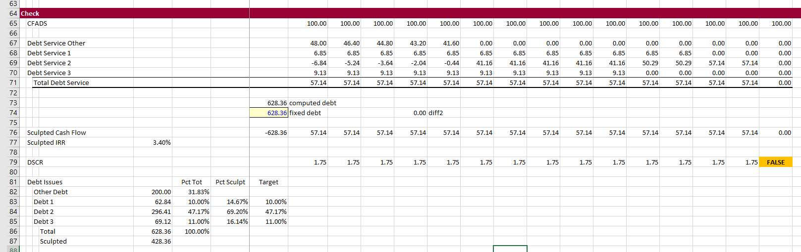
Step 5: Compute the Debt IRR from the Cash Flow of each issue and the total debt amount for each issue. This is the place I go wrong the most. Be careful and use the debt from the non-capture debt issues that is the debt commitment for the issue and defined as the percent of debt multiplied by the total aggregate debt. For the capture debt issue, use the NPV of the net debt service. That is the debt service from dividing the CFADS by the DSCR and subtracting the other debt service. Use the debt service from the individual issues and use the debt amount computed for the two issues from the PV calculations. You will have to move the debt amount to the period right before the COD using a flag. This is illustrated in the screenshot below where the IRR is computed. Note that there is a circular reference from this calculation and you must fix the IRR before you bring it to the top.
.

.
Results of a case with changing interest rates and also a debt issue with non-sculpted debt is shown in the screenshot below. For this case, the non-sculpted debt service is included in the subtraction from the capture debt issue. To implement the changing interest rate, use the SUMPRODUCT function with and interest rate index.
LEGACY — I Will Remove
1. Simple Allocation of Cash Flow Method to Compute Sculpted Balances
To introduce the issue I have created a simple example with three debt issues. Each issue has a different debt tenure and a different interest rate. Each issue also has a target amount as percent of the total debt. This set-up of the sculpted debt inputs is shown in the screenshot below. If there is a loan from a development financial institution, this type of situation with multiple debt issues that are sculpted can occur. If there is also a non DFI, the non DFI may have a shorter tenure and a higher interest rate. Note that the last debt issue in the screenshot has a tenure of 14 years while the first issue has a tenure of 8 years.
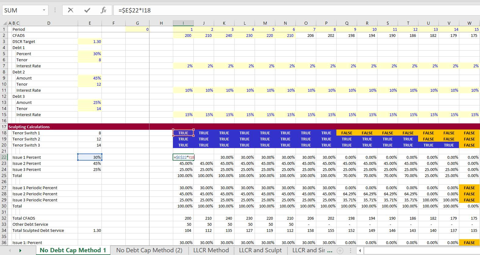
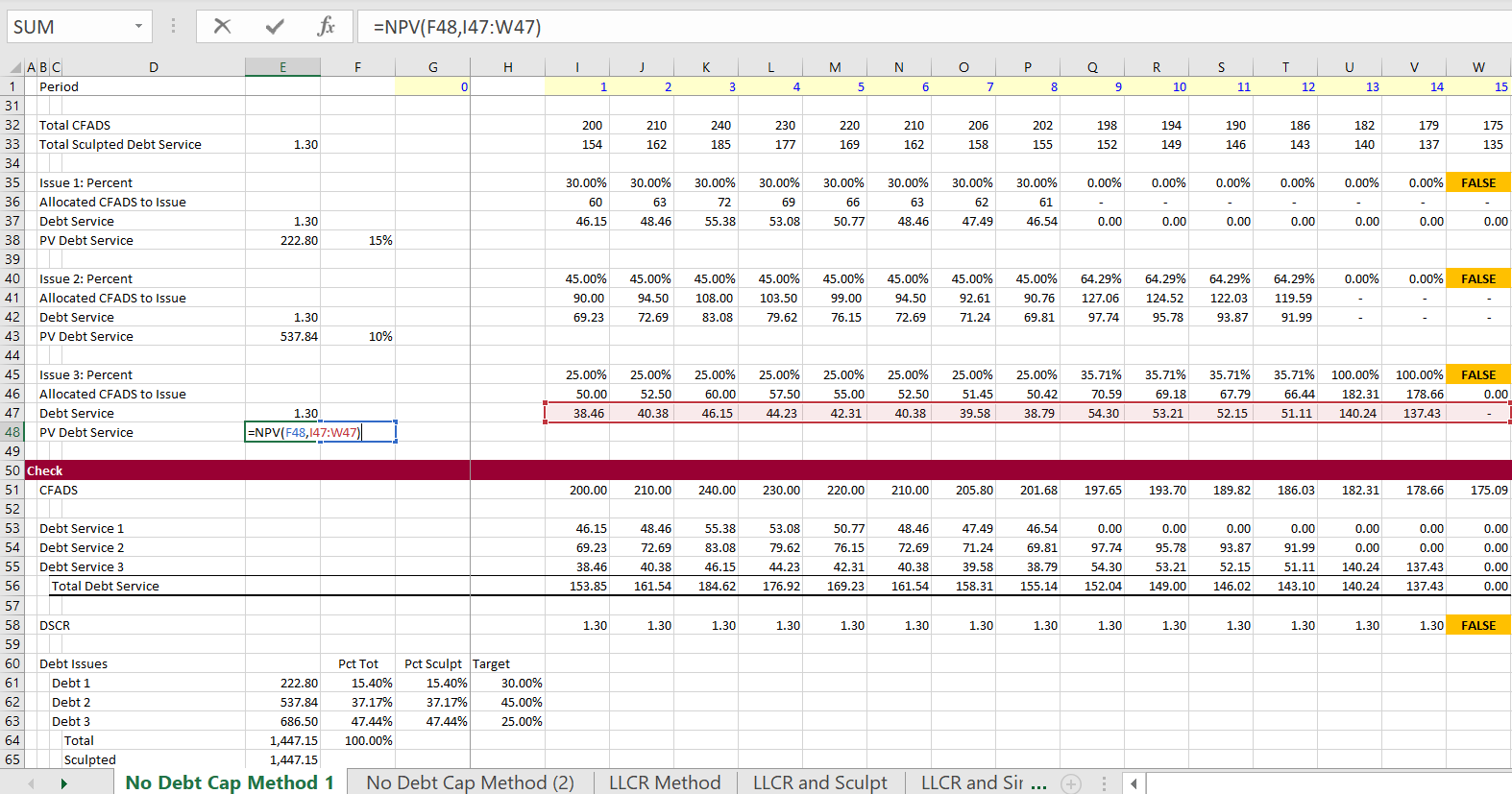
In the above screenshot, I entered the target sculpting for each debt issue. This had to be computed twice to recognize that after the first debt is finished, the percentages will change. Ultimately, when there is only one debt issue outstanding, all of the cash flow is allocated to that issue. These percentages are applied to the CFADS and then the sculpting is made with the normal NPV formula. The calculation of sculpting from the allocated CFADS to each issue is shown in the screenshot below. The NPV of the debt service gives you the total amount of debt as usual. If the interest rate is lower the NPV of the debt is higher. If the tenure is longer the NPV is higher. All of this means that the target percentages do not equal the final debt balance percentages. This is demonstrated at the bottom of the page. On the table at the bottom of the page, the target percentages computed from the NPV of debt service are very different from the target percentages.
2. LLCR Method to Allocate Sculpting for Multiple Debt Issues
I have described how you can compute sculpting if the debt balance is given. In this case you can use the formula to find the target DSCR to sculpt from a simulated LLCR. The formula is:
LLCR = PV(CFADS)/Debt
In the example below, the total debt is given as a fixed amount of 900 and it is allocated between three debt issues. For each issue, the PV of cash flow over the tenure of the debt is computed. Then, the total debt of 900 is allocated among the three issues. This defines the target amount of debt. The LLCR is computed for each issue from the PV of Cash Flow as well as the target amount of debt. This computation of the LLCR is illustrated in the screenshot below. The formula in the screenshot illustrates how you can put a formula (with TRUE/FALSE multiplied by the CFADS) into the NPV formula. Note that the LLCR is very high because the total cash flow is compared each separate debt issue.
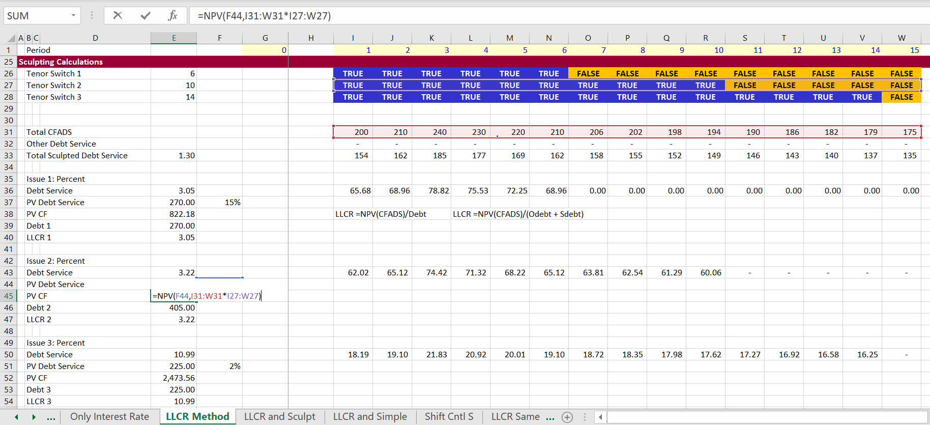
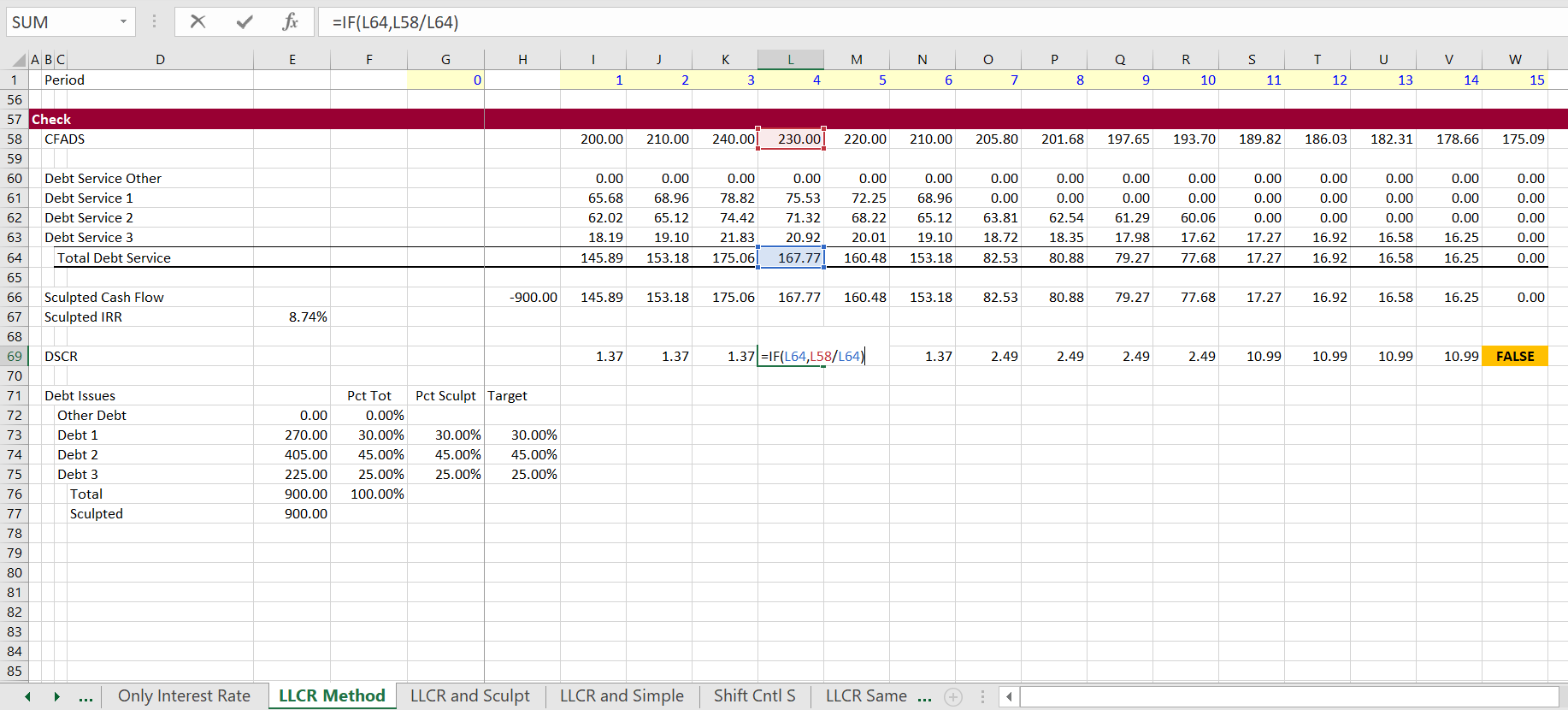
Results of the LLCR method are shown in the screenshot below. In this screenshot the good news is that the amount of debt is the target debt. But don’t get too happy. The very bad news is that the DSCR does not match either the LLCR on the overall debt or the target DSCR. Note that the DSCR begins at a level of 1.37. But after the first debt issue is finished, the DSCR increases to 2.49. Then, when only the last issue is outstanding, the DSCR is 10.99. If you allocate debt in this way the fact that the DSCR is not constant demonstrates that the method does not work.
3. LLCR on One Issue and Remainder Formula for Second Issue
The next method is getting a bit closer, but it still does not quite work. In a case with different interest rates and only two debt issues, you can reach both the target DSCR and the target percentages of debt. The method starts by establishing the overall debt size from the target DSCR. The debt size is derived by computing the NPV just like in any of the debt sizing cases. This interest rate is used in the formula Debt = NPV(Debt IRR, Debt Service) where Debt Service = CFADS/Target DSCR. But to compute the debt size, you need a discount rate. The discount rate is the overall IRR on debt is computed from evaluating the total amount of debt versus the debt service from all of the debt issues.
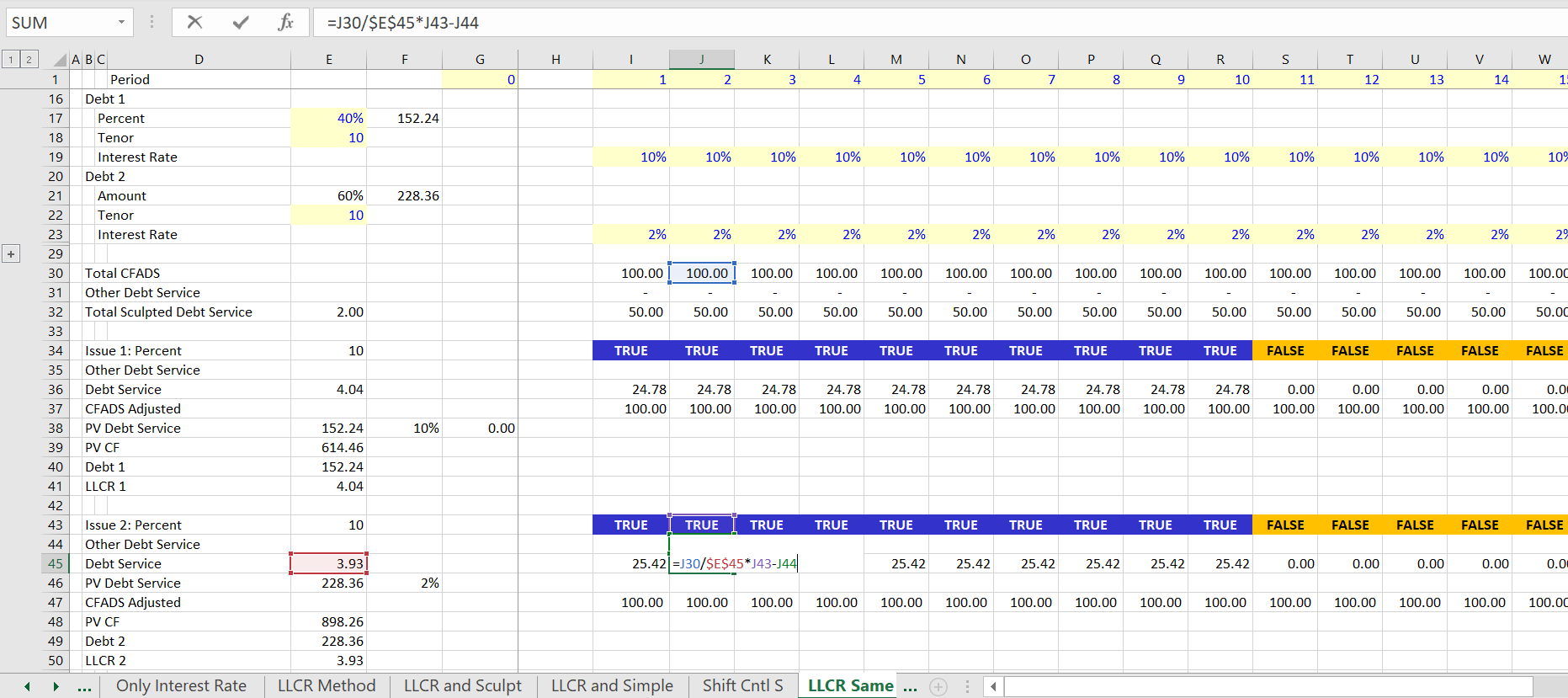
The method of establishing the LLCR fror one issue and using the debt service formula for the second issue works when the tenure is the same for both issues because of a circular reference problem. The screenshot below illustrates the approach. The first debt issue is computed with the LLCR using the method discussed in the prior section. The PV of cash flow is computed and then the LLCR is derived from the target amount of the debt: LLCR = PV Cash/Debt. Using this LLCR to compute debt service produces debt service for the first debt issue and it also yields the target debt size for the first issue. For the second issue, the formula for debt service of is DS = CFADS/DSCR – Other DS, where the Other DS includes the debt service from the first debt issue. I label this debt issue as the capturing debt issue. When you compute the NPV of this cash flow for the second issue, you get the same amount as the target debt percent multiplied by the total debt.
A complexity with this method is that works from the IRR on the overall debt. This is needed because the IRR on the debt that is used for sculpting. But the IRR on debt cannot be computing until the debt issues are evaluated. This causes a circular reference which will be discussed in detail below. This is shown in the second screenshot below.
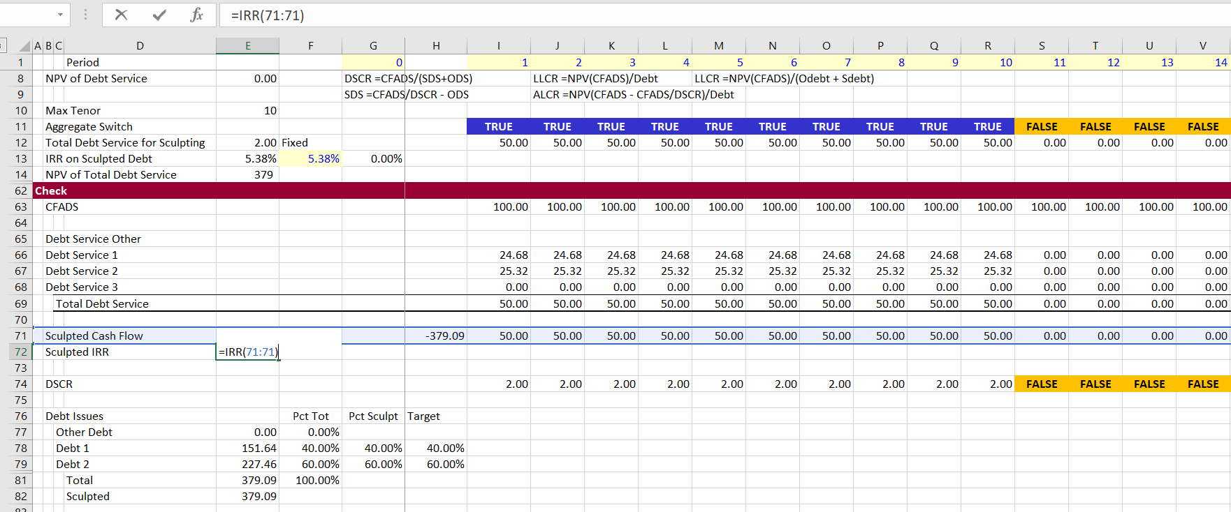
The next screenshot demonstrates the results of this combination of LLCR and formula method. In this method, the target DSCR of 2.0 is achieved and the target debt amounts for the two issues are also achieved as shown on the bottom of the screenshot. To make this computation work, the debt IRR is computed from the debt service of the two debt issues. This IRR is 5.38%. But the IRR is not known until the debt service of the two issues is computed. The IRR is copied and pasted into the calculation for the NPV of overall debt service.