This page demonstrates my method for creating formula evaluation. I have created some VBA code that allows you to find the sources and explanation of a formula by pressing a single short-cut key. You can quickly go to different source cells; you can quickly find the sources of LOOKUP and SUMIF formulas; you can see the formula in descriptive terms; you can keep looking deeper and deeper into formulas, and you can do this all without using the blue precedent hours. I know there are other similar programs that do this and many of them are not free. But with the VBA code shown below, you can customize the presentation and what you really need. You also do not need any add-in; instead you just have to have the GENERIC MACROS program open. Alternatively, you can copy the VBA code that is described below into your own personal macros program. The GENERIC MACROS program is attached to the button below.
.
Instructions for Downloading Files with Macros
.
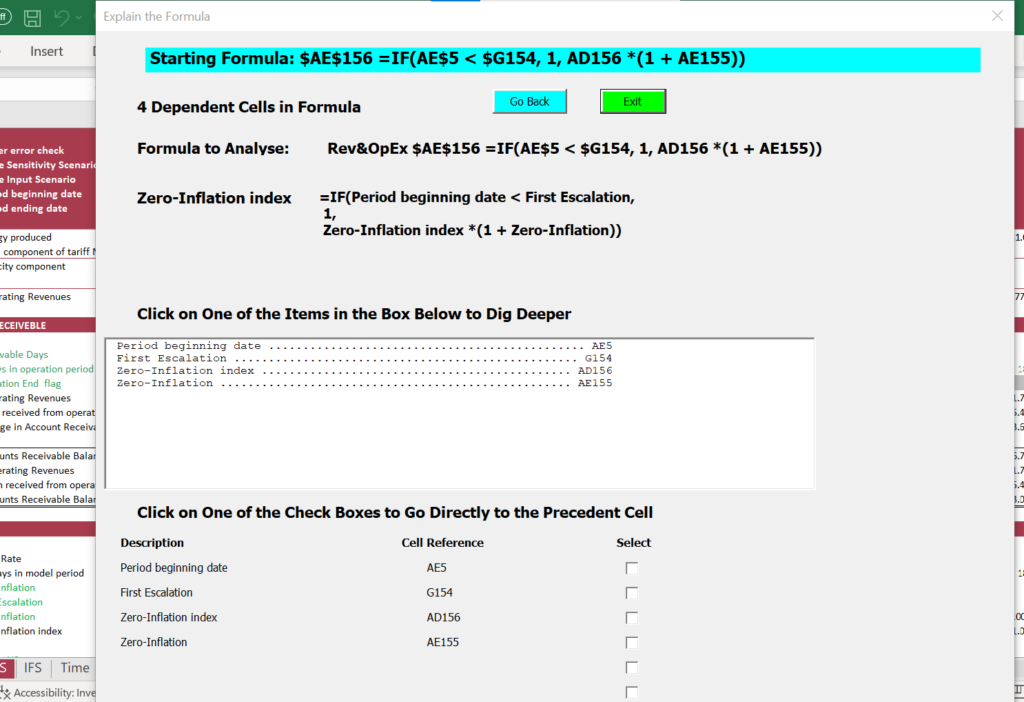
I originally made the program because the CNTL, [ short-cut is difficult to find on a German keyboard or an Italian keyboard. My friend Sasha who is a very good modeller told me he could not find the CNTL [ key effectively. I told him that I would try and create a simple short-cut. Well, the short-cut key is not at all easy to replicate with simply recording the CNLT [ key and it does not work. Further, the CNTL [ key kind of sucks. If you have a complex formula, it only gives you the first component; it does not at all help with LOOKUP, which is my favorite; it does not give you any descriptive information. So now when you open GENERIC MACROS and press the ALT, U short-cut sequence, you get the following screen (that you can easily modify). When you place yourself on a cell in excel and press the ALT and u sequence, you will get a screen that looks something like the screen below. Note that I am sure I will change this many times in the future and I am sure you can make the screen that comes from the userform much more artistic.
When you have this screen, you can click on one of the items in the list box and you will see a similar layout. You can also go to the bottom and then click on one of the cells to go to that cell just like if you used the CNTL [ short-cut in excel. Once you go to the cell you can also press the F5, just like if you were using the sequence CNTL [ and F5 in your model.
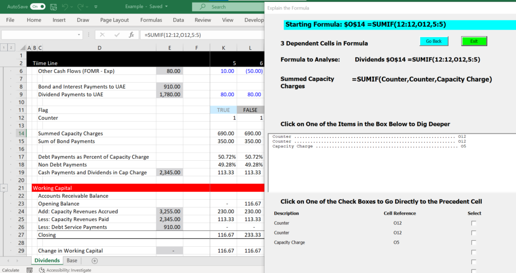
If you have a SUMIF or LOOKUP in your model, I made the program work a little differently. In this case, the screen shows the entire rows that are used in the formula. Again, the formula shows the description of what is happening. In the screenshot below, I have moved the userform around so you can see the original formula.
Using the Split Function
The message box below illustrates the results of using the SPLIT function which is useful in working with the range names. You can split using different delimeters
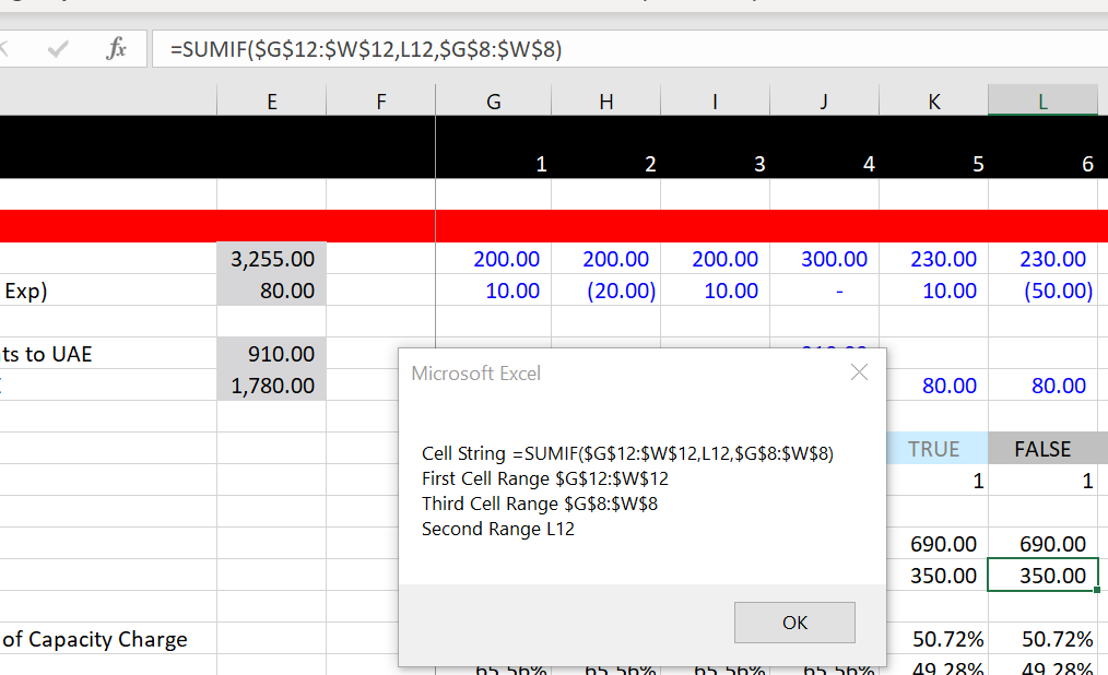
The message box that splits up the equation is created by the following VBA code. Note that you create an array to create these parts
             split_lookup = Split(cell_string_original, "(")
             split_inside_range = Split(split_lookup(1), ")")

             first_range = lookup_range(0)
             second_range = lookup_range(1)
             third_range = lookup_range(2)

             If debug_code = 12 Then _
                    MsgBox " Cell String " & cell_string_original & Chr(10) & _
                           " First Cell Range " & first_range & Chr(10) & _
                           " Third Cell Range " & third_range & Chr(10) & _
                           " Second Range " & second_range

             first_number_range = Split(first_range, ":")
             third_number_range = Split(third_range, ":")

             first_cell_range = first_number_range(0)
             third_cell_range = third_number_range(0)

             If debug_code = 12 Then _
                    MsgBox " First Cell Range " & first_cell_range & Chr(10) & _
                           " Third Cell Range " & third_cell_range & Chr(10) & _
                           " Second Range " & second_range
Step 1: Start of the Program. Get the Formula and then Test if it is a Formula
The first step is to define the formula. You can use the the ACTIVECELL.SELECT function. With this you can get the row and the column and then find the formula. The code just below shows how you can make sure to only do the whole thing if the cell is a formula — not a text; not an error; not a number. If this happens, just go to the end of the program.
ActiveCell.Select

row = Selection.row
col = Selection.Column

cell_string_original = Cells(row, col).Formula

' This is the start of everything.  Find the formula selected
If WorksheetFunction.IsText(Cells(row, col)) = True Then
GoTo finish_the_calculations:
If WorksheetFunction.IsError(Cells(row, col)) = True Then
GoTo finish_the_calculations:
If WorksheetFunction.IsNumber(Cells(row, col)) = False Then
GoTo finish_the_calculations:
Step 2: Use the Precedent Item and the SPLIT function to find Cells in the Same Sheet
‘—————————————————————————————————————-
‘ Part 1 — Precendents in the same sheet
‘—————————————————————————————————————-
    On Error Resume Next

    this_sheet_precedents = Cells(row, col).DirectPrecedents.Count ' This creates additional shapes; there is no error if no dependents
    total_cells_in_formula = Val(this_sheet_precedents)                ' start with teh total number of cells
    total_cells_same_sheet = Val(this_sheet_precedents)                ' start with teh total number of cells
    precedent_string = Cells(row, col).DirectPrecedents.Address
'
' Take out $ signs so can replace formula
'
For i = 1 To 30
temp_string = WorksheetFunction.Substitute(precedent_string, "$", "", 1)
precedent_string = temp_string
Next i

For i = 1 To 30
        temp_string = WorksheetFunction.Substitute(cell_string_original, "$", "", 1)
        cell_string_original = temp_string
    Next i

    precedent_array = Split(precedent_string, ",")                ' This is a key formula that separates the array
Step 3: Compute the Outputs in Case where Cells are on the Same Page
‘
‘ Once you have the precendent array defined, you can put together the output strings
‘
    target_length = 70
    one_period = "."
    total_period = ""

    For found = 1 To total_cells_in_formula
        total_period = ""                                                  ' set the cell for periods to zero
        cell_range_found(found) = precedent_array(found - 1)               ' the name of the cell
        row_of_range(found) = Range(cell_range_found(found)).row

        For j = 1 To 10                                                        ' Go around 10 columns
            If WorksheetFunction.IsText(Cells(row_of_range(found), j)) Then
                string_found(found) = Cells(row_of_range(found), j).Value
                display_string(found) = string_found(found) & "" & cell_range_found(found)

                temp_length = Len(display_string(found))       ' this is to derive the number of dots or spaces
                added_length = target_length - temp_length     ' this is the number of dots to add

                For k = 1 To added_length                      ' go around one by one and add the dots
                   total_period = total_period & one_period    ' creates a string with dots
                Next k
                display_string(found) = string_found(found) & " " & total_period & " " & cell_range_found(found)

                Exit For
             End If
        Next j
    Next found
Step 4: Compute the Number of Explanation Points to Find Cells in Other Sheets
‘————————————————————————————————————
‘ Count the exclamation points for range names in other sheets
‘————————————————————————————————————
       number_of_exclamations = 0
       exclamation(1) = 2

       cell_string_test = cell_string_original

       For i = 2 To 10
            exclamation(i) = 0
       Next i

       For i = 2 To 10
‘
' On Error GoTo end_of_exclamation_loop: ' Note how the error trap does not work'
On Error Resume Next
     exclamation(i) = WorksheetFunction.Find("!", cell_string_test, exclamation(i - 1) + 1) ' seems to convert ; -- look after the first argument
If exclamation(i) = 0 Then Exit For
If exclamation(i) <> exclamation(i - 1) Then number_of_exclamations = number_of_exclamations + 1
Next i
       total_cells_in_formula = total_cells_in_formula + number_of_exclamations               ' start with teh total number of cells

       If number_of_exclamations > 0 Then

         start_count = total_cells_same_sheet
         found_count = start_count