This page demonstrates how you can solve project finance issues in some complex cases such as replacing the DSRA with a letter of credit; adding balloon payments in sculpting; including an equity bridge loan during construction, computing the CFADS or the debt service with changes in the DSRA; including pre-commercial cash flow in the project and other issues. To evaluate these issues I have created a model that you can use as a basis to evaluate the issues. I show you how to add the UDF model to the analysis.
Example of Project Finance Model with Parallel Model to Resolve Circular References
The model that you can download by clicking on the button below resolves circular references without the iteration button or copy and paste macros. This makes the model faster, more transparent, more accurate and much more flexible. I have been working on this for a long time and I am going to post a template model that makes it easy to add to your model that has circular references. Please do not think this is difficult to do as I will be adding a lot of examples and videos that demonstrate you can easily add a page to your model and get rid of your copy and pasted values. You can add up to 30 different debt issues; you can use all kinds of different debt sizing, debt funding, debt repayment and interest rate structures. You can put in balloon payments, you can sculpt where changes in the DSRA are in the numerator or denominator of the sculpting formula.
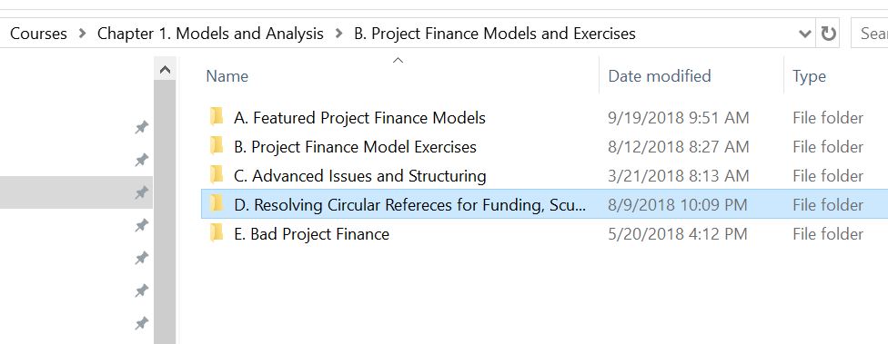
I am continue to perfect this approach so it is easy to implement and can handle more possible of debt and taxes. You can see my progress if you have downloaded the google drive. The location of the files on the google drive is demonstrated in the screenshot below.
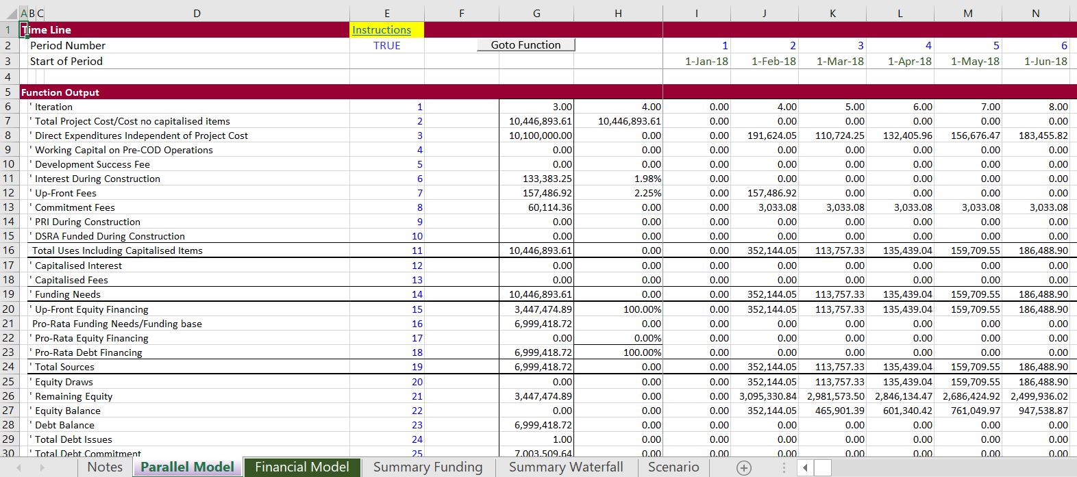
The screenshots below illustrate a few concepts about what the parallel model concept can do. The first screenshot demonstrates the parallel model page that you add to your model. This has a model that can be entirely independent of your model and used to test the accuracy of your model (the A in FAST). Data from the parallel model like the CFADS, total funding and DSRA flows can be connected to your model. This will eliminate the circular references in your model and make your model more transparent (T in FAST). By solving the circular references your model will be much more flexible and fast (the F in FAST). Finally, the parallel model outputs are structured so you can see all of the key cash flows of during and after construction. Making the parallel model in the two screenshots is done with a template and you do not have to re-enter the stuff.
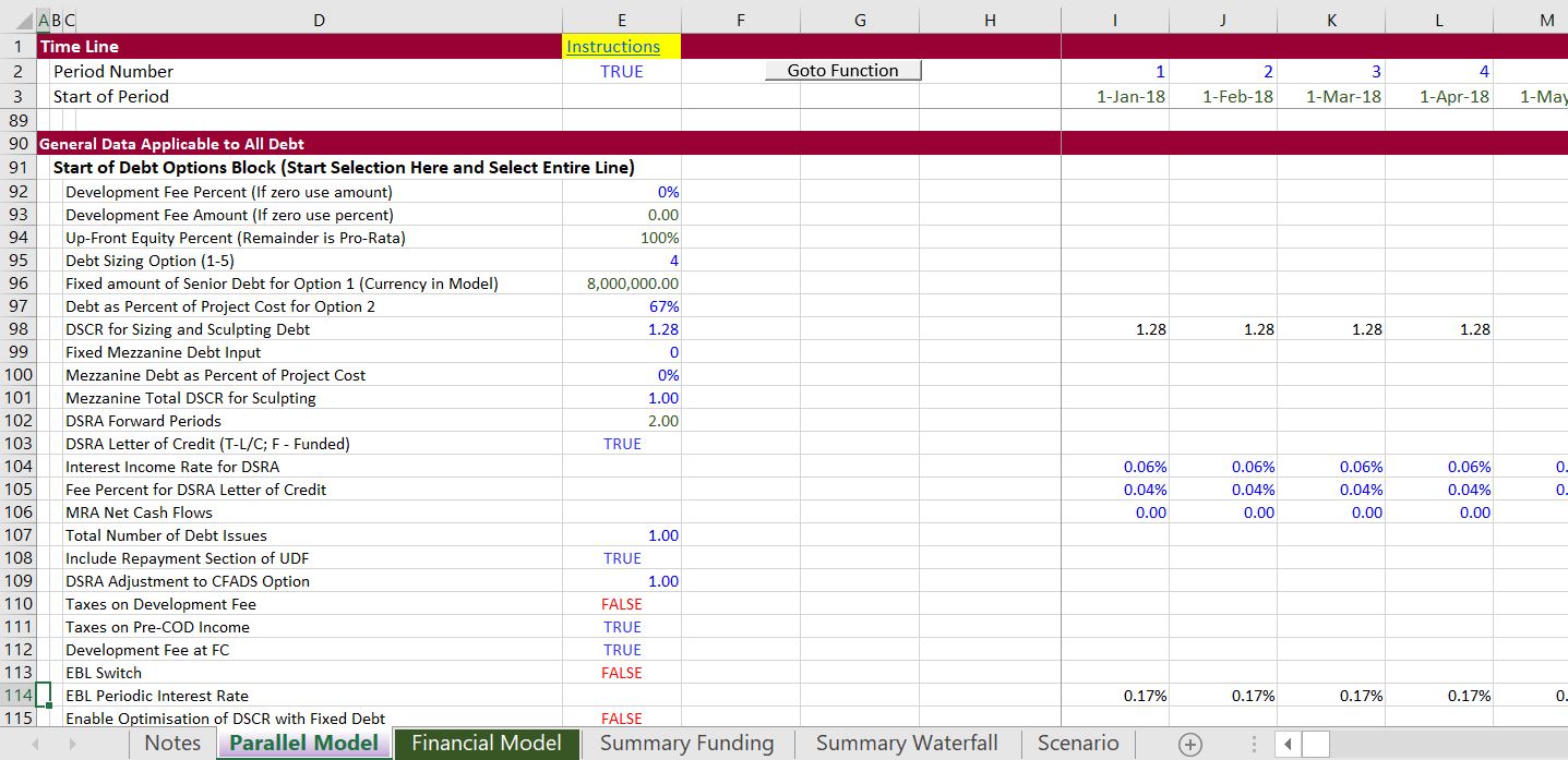
The screenshot below illustrates some of the inputs that you put in the parallel model. Please note that all of these inputs come from somewhere in your model. More importantly, many of the inputs that you may not care about like withholding taxes on debt issues or the percent of EBITDA cap on tax can be left out. It should only take you a couple minutes to fill in the inputs. Note that some of the inputs are scalar variables with single inputs while other variables are time series variables that some people simply call time variables.
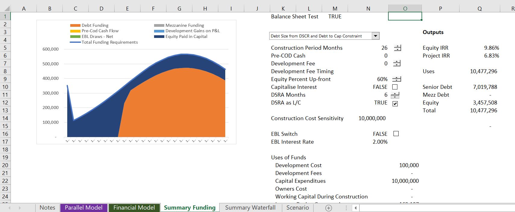
The next screenshots demonstrate some of the things that you can do with the parallel model concept that you could hardly imagine if you were using a copy and paste routine. The examples do not show that you can use a goal seek when you change anything (i.e. you can find the required price to give you an IRR with different structures. The first screenshots illustrate the types of funding analysis that you can do. In the first example there is equity first funding.
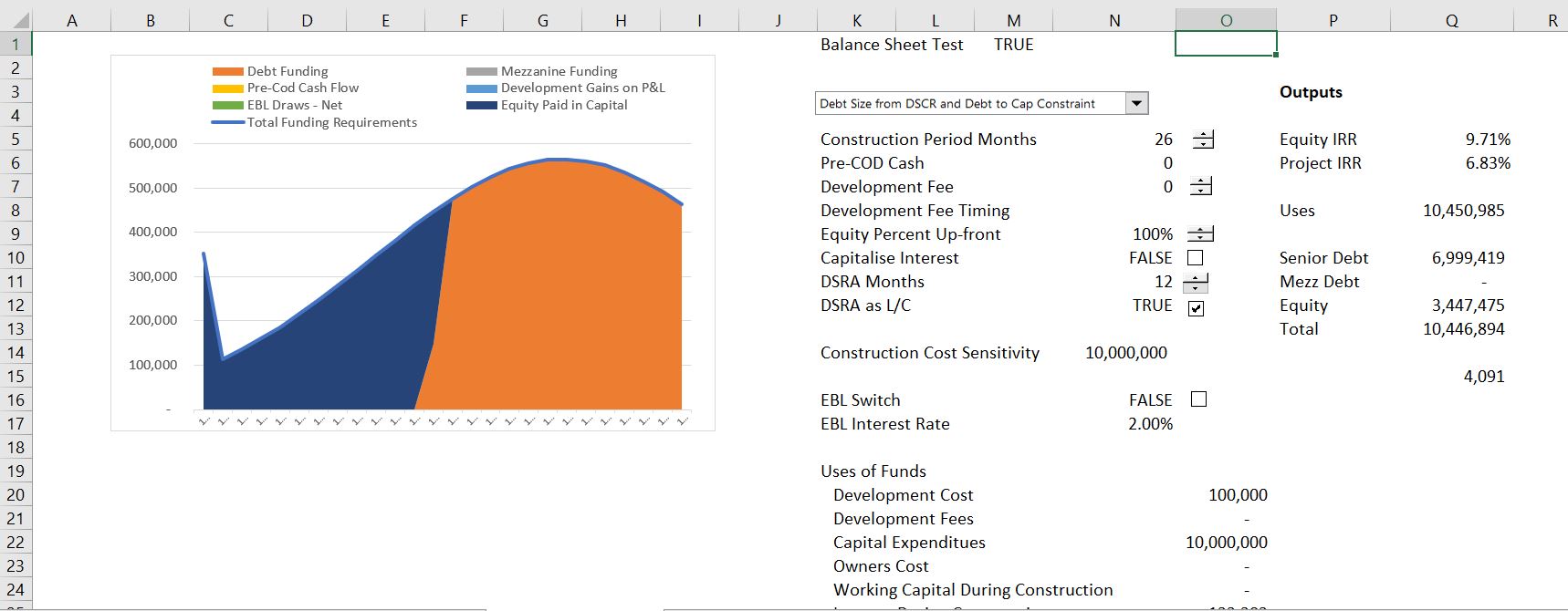
The second example shows what happens when you click the EBL switch button. In this case the is funded by a loan with an interest rate of 2%. Note that even with a short construction period of 26 months, the equity IRR increases from 9.71% to 10.66%. There is no copy and paste routine to run, there is no time to wait.
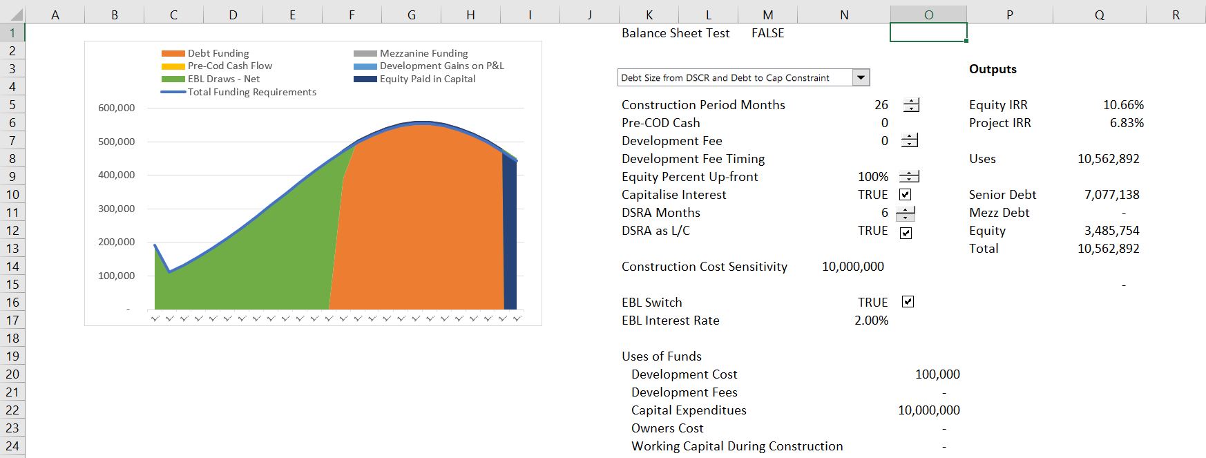
The third screenshot of the summary page shows the case where a part of the funding is from equity up-front and a part is funded using a pro-rata funding. This causes a lot of circular reference, but you can use the spinner button and change the equity up-front percent. You can immediately see what happens to the equity IRR.
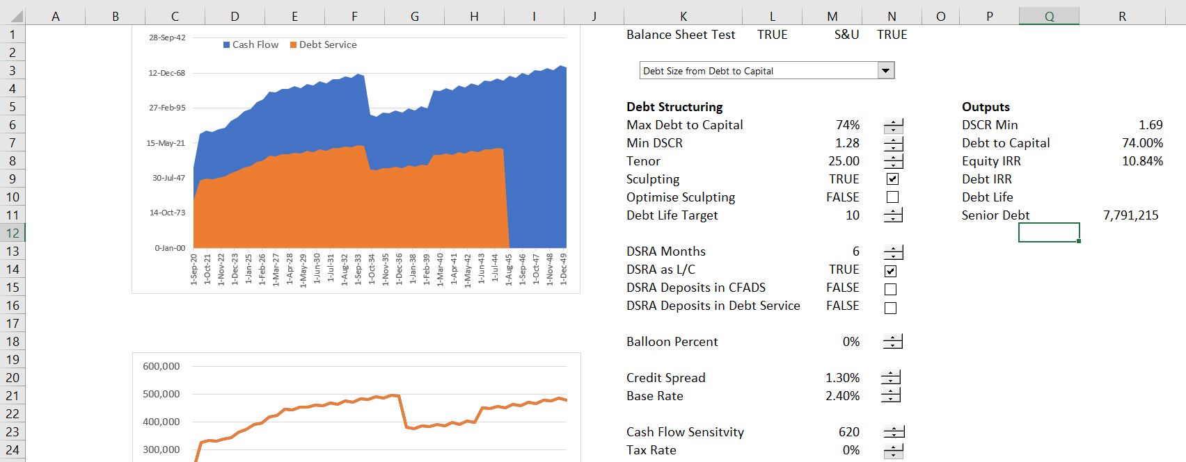
The next screenshots demonstrate how the parallel model can be used to make your model flexible in presenting results during the repayment periods. The graph shows cash flow and debt service. In the first demonstration a fixed amount of debt is used from the option. The parallel model allows you use different assumptions — fixed debt, debt from debt to capital, debt from DSCR or debt from minimum criteria — without pressing circular reference buttons.
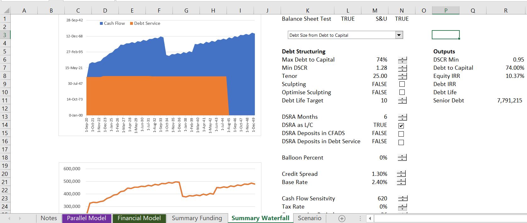
The next screenshot demonstrates that you can change the repayment from sculpting a repayment schedule input. In this case, you can see the effect on the DSCR and the equity IRR from different assumptions. Again all of this stuff can be incorporated in your model by adding a parallel model page and using the template.
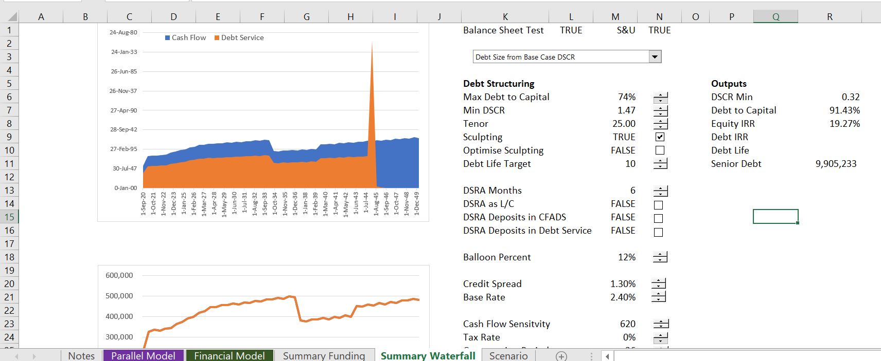
The third picture of the results of the model illustrates what happens when you change the debt sizing method to DSCR.
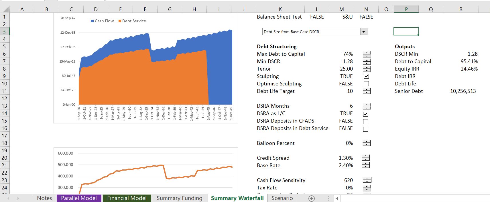
The next screenshot shows the effect of using the DSRA changes in the DSCR for sculpting. The DSRA changes could be classified as part of the numerator or a deduction in the denominator. If you tried this with a copy and paste routine you would end up with a real mess. The parallel model can apply different DSRA techniques by applying some mathematical formulas rather than forcing things. If you look carefully at the screenshot you can see that DSRA deposits in debt service is checked, meaning that the DSRA changes are included in the denominator of the DSCR for sculpting purposes.
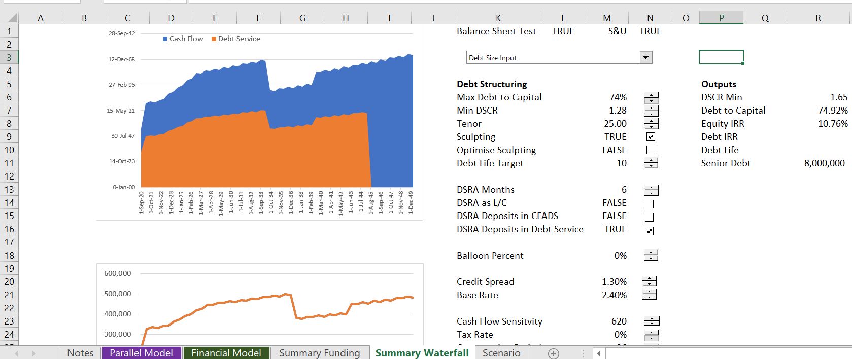
The final screenshot demonstrates the effect of a balloon payment. If a balloon payment is used, there will be more debt for the given DSCR. This will have a different effect if equity up-front is used or the DSCR is used to finance the debt. There are painful circular references from the balloon payments as with the other factors.
Circular Exercise 1 – Fee Exercise.xlsm
circular functions 2.xlsm
Circular Exercise 7 – Fees.xlsm
Circular Exercise 1 – Cash Flow Sweep without Taxes.xlsm
Circular Reference 2 – Cash Sweep.xlsm
Bridge Loan Circular Exercise.xlsm
Circular Exercise 6 – Resolving Funding 1.xlsm
Exercise 26 – Funding Cascade and Circularity.xlsx
Circular Exercise 6 – Resolving Funding 2.xlsm
Circular Reference 2 – Cash Sweep.xlsm Circular Exercise 8 – DSRA.xlsm
IDC and Circularity with Real Estate.xlsm
IDC and Circularity with Real Estate – Copy and Paste.xlsm
IDC and Circularity with Real Estate – Function.xlsm
| Excel Exercise File | Video | Chapter Reference | Page Reference | ||||||