This page explains how to create a model that has normalisation of terminal cash flow consistent with terminal growth assumptions. Two different methods are explained that provide a normalised ration of capital expenditures to depreciation. The first method accounts for the depreciation life and the terminal growth rate. The second method incorporates the projected life and the depreciation life and also the historic growth in capital expenditures which drive the replacement of existing assets. User defined functions that define the stable amount of capital expenditure to depreciation given a couple of inputs for terminal growth, depreciation rates and in some cases historic growth. A very basic idea in life is that you have to make an investment to achieve something good. In the context of terminal value, if the growth in terminal cash flow is higher, the capital investment must also be higher. This means that the projected normalised capital expenditures cannot be independent of the level of growth.
- If you are assuming a higher rate of growth in EBITDA, you must assume a higher level of stable capital expenditures. This should be obvious.
- You also need to replace existing assets at some time if the EBITDA is to continue.
- The growth includes growth from inflation as well as real growth.
- You can make a little growth and depreciation analysis to evaluate how what happens to the stable ratio of capital expenditures to depreciation, where the depreciation reflects the status of existing assets.
The basic method without considering historic growth is shown in the code below. All you have to do is copy this code into your excel workbook (but since Option base 1 is at the top, make sure it is at the top of a module page). Then you have a function that will give you the capital expenditures to depreciation as a function of the depreciation life and the growth rate. You can also use a timing switch.
.
Option Base 1
Function cap_exp_depreciation_simple(life, growth, Optional timing_code)

If IsMissing(timing_code) Then timing_code = 1

base_capexp = 100
capexp = 100

plant_balance = 100

For i = 2 To life + 1

capexp = capexp * (1 + growth) ' Capital Expenditure After Depreciation
If i = life + 1 Then retirement = base_capexp

If timing_code = 3 Or timing_code = 2 Then _
    plant_balance = plant_balance + capexp - retirement ' Closing Balances

depreciation_exp = plant_balance / life ' Depreciation on Opening Balance
If timing_code = 2 Then depreciation_exp = (plant_balance - (capexp - retirement) / 2) / life ' Depreciation on Opening Balance


If timing_code = 1 Then plant_balance = plant_balance + capexp ' Closing Balances

Next i

cap_exp_depreciation_simple = capexp / depreciation_exp


End Function
.
The next function below that you can also copy is a more complex function where you reflect the historic growth rate of the corporation as well as the life and the projected growth rate. The output again is the stable capital expenditures to depreciation.
.
Option Base 1

Function cap_exp_depreciation_simple(life, growth, Optional timing_code)

If IsMissing(timing_code) Then timing_code = 1

base_capexp = 100
capexp = 100

plant_balance = 100

For i = 2 To life + 1

capexp = capexp * (1 + growth) ' Capital Expenditure After Depreciation
If i = life + 1 Then retirement = base_capexp

If timing_code = 3 Or timing_code = 2 Then plant_balance = plant_balance + capexp - retirement ' Closing Balances

depreciation_exp = plant_balance / life ' Depreciation on Opening Balance
If timing_code = 2 Then depreciation_exp = (plant_balance - (capexp - retirement) / 2) / life ' Depreciation on Opening Balance


If timing_code = 1 Then plant_balance = plant_balance + capexp ' Closing Balances

Next i

cap_exp_depreciation_simple = capexp / depreciation_exp


End Function
.
Evaluating Capital Expenditure to Depreciation With Difference in Historic Growth and Replacement of Assets
Consider population. If there was a baby boom with a lot of births and you must replace the births. Then there will be a second cycle when the baby boom comes to the age when they have children. In a similar but not exact way, if you are replacing EBITDA and you made a lot of capital expenditures, one day you will have to either allow the EBITDA to decline to nothing or replace the capital expenditures. The problem is that these are not smooth. Further, tying to levelize out the capital expenditures is tricky.
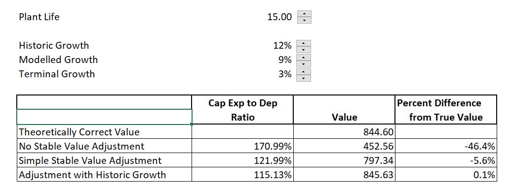
The table below illustrates the effects of different historic growth rates. Note that incorporation of historic growth does somewhat improve the valuation. In the file there is a theoretically correct value and then the different methods of measuring capital expenditures in the terminal value are applied. The method of not including any adjustment is dramatically wrong.

You can think of a case where you have made more capital expenditures in the past. Then you have to replace the capital expenditures to maintain the EBITDA. But the depreciation expense is also higher even though the expenditures were made.

[wonderplugin_video iframe=”https://www.youtube.com/watch?v=-NUeYz_wm04″ videowidth=600 videoheight=400 keepaspectratio=1 videocss=”position:relative;display:block;background-color:#000;overflow:hidden;max-width:100%;margin:0 auto;” playbutton=”http://edbodmer.com/wp-content/plugins/wonderplugin-video-embed/engine/playvideo-64-64-0.png”]
This function shows how to evaluate the adjusted capital expenditures if you have an idea of what the is the historic growth. You can copy this function into your model.
.
Option Base 1
Sub depreciation_Rate_functions()

End Sub


Function adjusted_cap_exp(historic_growth, future_growth, life, wacc)

Dim cap_exp(1000)

gross_plant = 1

method = 1
' method 2

If method = 2 Then
base = gross_plant / life
End If

If method = 1 Then
base = find_base(historic_growth, life)
End If


If life < 0 Then Exit Function

cap_exp(1) = base

total_test = base

For i = 2 To life

Select Case method:

Case 1:
cap_exp(i) = cap_exp(i - 1) * (1 + historic_growth)
Case 2:
cap_exp(i) = cap_exp(i - 1)
Case 3:
cap_exp(i) = cap_exp(i - 1) * (1 - historic_growth)

End Select

total_test = total_test + cap_exp(i)

Next i

' MsgBox " base " & base & " total test " & total_test


opening_balance = gross_plant

pv_factor = (1 + wacc)

For i = life + 1 To 500

pv_factor = pv_factor * (1 + wacc)

closing_balance = opening_balance * (1 + future_growth)

retirement = cap_exp(i - life)
cap_exp(i) = closing_balance - opening_balance + retirement
depreciation = opening_balance / life

pv_cap_exp = pv_cap_exp + cap_exp(i) / pv_factor
pv_dep = pv_dep + depreciation / pv_factor

opening_balance = closing_balance

Next i

adjusted_cap_exp = pv_cap_exp / pv_dep


End Function

.
Stable Deferred Tax
The file that you can download below includes analysis of stable deferred tax changes as deferred tax changes should be in cash flow and not in the bridge between equity value and enterprise value.
Simulated Depreciation Expense and Retirements
Excel File with Simulated Depreciation Expense Analysis and Varying Long-term Growth Rates