This page describes how to build a corporate model on a step by step basis and at the same time describes some of my theoretical ideas about each parts of building a model. The step by step guide for corporate modelling includes background on value and economic activity; alternative ways to put historic data into your models and assess performance; methods for developing and presenting assumptions; constructing models in a structured and transparent manner; adjusting depreciation for asset retirements and changing growth; computing free cash flow and developing alternative valuation methods; and, addressing advanced issues including circular references and stable capital structures. In explaining the different steps for creating a model I use a few examples from India.
Like other pages, I have created this page as an adjunct to my teaching activities. My general teaching objective is to give participants a few ideas on both theory and practice that you will actually remember. In a class, you may forget the details but I hope that you will have a vague memory of a few key practical and theoretical details (and that you will be interested enough in the class to keep off you phones). So that you can remember details that you forget in classes, I put together the details of the corporate modelling in separate paragraphs, downloadable files and videos. Teaching style is to leave you with videos and resources. In the discussion below, I have provided links to other pages that detail.
Section 1: Some Introductory Philosophical Points about Modelling, Long-term Stock Prices and Growth
For each of the sections below below I present a few elements of theory and practice associated with different parts of corporate modelling. In this first section I introduce some fundamentals of potential growth in earnings, expected returns and volatility with analysis of stock prices. For each of the steps I introduce some theory and practical ideas that I hope will make you think about corporate modelling and valuation a bit differently.
Theory: Small differences in IRR make a big difference in value over the long-term; projecting cash flow and risk for value; beta and volatility are closely related; returns and economic growth and income distribution; earnings in recessions and ability to maintain growth; market returns and bond returns over the long-run; CAPM B.S.; relationship between volatility, returns and beta; real and nominal returns and adjustments.
Practice: Examples of actual models; making flexible graphs; computing returns with IRR and growth; using TRUE/FALSE to make flexible analysis; NA trick with graphs; generic macros and contents;
Theory of Stock Prices, Macro Economics and IRR
To demonstrate some general ideas about valuation and modelling, I use the comprehensive stock price and economic activity database (you can find more information about how to use this at associated link). The graph below illustrates stock returns, economic growth, and bond returns for a long-term period (since 1957). The IRR next to the graph can be called the TSR and measures the compound growth for the various series (that is what the IRR measures and it is in inflation adjusted terms). I would like you first to think about a couple of issues with respect to this workbook and the screenshot below. First, notice the small difference in the inflation adjusted returns makes a very big difference in the final amount of money. When you make your valuations or think about things like country risk premiums or small company adjustments to WACC or cost of capital, that is why seemingly small differences make a big difference in value (see the link). Note also that the returns above inflation are not very high (the WACC calculator that throws around different WACC’s is incredible rubbish). Expecting to earn high returns when you measure the WACC can be very silly. Further, you should not be surprised that small differences in WACC make a big difference in value. You can also think about volatility and how much the volatility has changed over time. Think about how you need a premium for the volatility. But if you need a volatility and corporate profits are a higher percent of GDP, something has to give.
.

.
Stock Prices of Individual Companies, Value and Risk
Now you can look at a couple of stocks I used some stocks from India and compared them to European or U.S. stocks. To do this you need to make sure the currency is consistent — yahoo reports stocks in different currencies and indices are generally expressed in the local currency. This means that to make a reasonable comparison some of the series must often be adjusted. To evaluate corporate value, I have a picked a few stocks from India — HT Media, Tatar Motors and Reliance.In the long-run the stock values are driven by earnings and cash flow. They are of course affected by expected future cash flow and risk. The screenshot shows that HT Media had a decline in stock price; Tata motors had an increase and then a decrease in price; and Reliance had an increase in price. The right hand side of the screenshot shows the accumulated returns from investing in different stocks over the period. These numbers are converted to USD so you can compare the returns in common currencies. Notice that if you invested in the US stock market, you would have doubled your money over the period. If you invested in the Indian stock market, you would receive 1.36 on every dollar you invested. For Reliance you would have go 3.22 — this is the implication of an IRR 10.87%.
.

.
Exercise with Stock Price Data
.
I will emphasise in the course that all you need in terms of excel functions is INDEX, LOOKUP and AVERAGEIF in the associated link. With these few functions you can compute compute returns, beta and volatility. This is easy when you use the LOOKUP function (not VLOOKUP or HLOOKUP please). I introduce you also to AVERAGEIF which will be useful in presenting historic valuation multiples. A couple of short-cuts and EIA and Shift, CNTL R. Also stop wasting time on formatting and colours and use the financial tools. You can review the remind yourself how to use the GENERIC MACRO file in the associated link. You can review the effective short-cuts like ALT, E, I, S in another link.
.
Comprehensive Stock Price, Commodity Price, and Economic Series Database with Monthly Prices
.
[wonderplugin_video iframe=”https://www.youtube.com/watch?v=JfZyk7HuTSU” videowidth=600 videoheight=400 keepaspectratio=1 videocss=”position:relative;display:block;background-color:#000;overflow:hidden;max-width:100%;margin:0 auto;” playbutton=”http://edbodmer.com/wp-content/plugins/wonderplugin-video-embed/engine/playvideo-64-64-0.png”]
.
Section 2: Acquiring Data and Evaluating ROIC and Growth
This section begins the real discussion of modelling. The very real world problem of efficiently getting financial statement and other data into your models is addressed along with what is the first thing you should do when you get the data. I suggest that the real task in modelling at the end of the day is forecasting whether a company can gain, lose or maintain its monopoly power and what that means in terms of value. You can see this with the consultant matrix where businesses can move from the powerhouse box to the throwing away money box. I address the free cash flow to the firm versus free cash flow to equity and illustrate problems with the value driver formula.
Theory: Return and growth; using ROIC rather than ROE to measure fundamentals of the business and ask tough questions about maintaining ROIC; ROE versus ROIC in assessing financial model; problems with ROIC in practice; reconciliation of ROI and IRR; ROI and growth versus cost of capital; real issue — when will companies develop monopoly power and if they have monopoly power, how long will it last; problems with McKinsey formula for ROI growth and value; fundamental NPV rule and growth versus ROIC; Examples of stupid ideas: S&P growth forecasts; using the McKinsey formula
Practice: Acquiring data with WORKBOOKS.OPEN and Indirect to measure return. Reading PDF to get financial data and measure returns. Using the SUMPRODUCT with -1 and +1 to reconcile ROIC and see how much investment has been made in the fundamental business. Graphing scatter plot and advanced F11 rules. Interpolate tool and lookup function. Using macros instead of data tables.
Theory of Value Drivers with ROE, ROIC and McKinsey Model
In using a financial model to compute value, the ultimate issues is whether the company being valued is making good investments and growing. If the company earns a little or a lot more than its cost of capital, the company should grow and it should have a relatively high value. When you boil things down, the financial is about forecasting returns and growth and assessing risk. When applying the value principles, the difference between the ROE and ROIC is not trivial and related to some kind of financial theory. ROIC should do something crucial, and that is to measure the returns from the core business of the company. That is, without pollution of the effects of things like having a whole bunch of cash on the balance sheet or investments in other associated or non-associated companies or making money from changes in the value of derivatives and other financial instruments.
A little financial mathematics will be reviewed so you can prove the formula P/E = (1-g/ROE)/(k-g). But the model does not work when you have changing parameters and in particular, you cannot assume that return converges with the return in the terminal period. You have to think about things instead. Further discussion of how to use the value driver principles in different situations is discussed in the associated link. The screenshot below illustrates how growth and returns affect value using a scatter plot where a series of different returns and growth rates are simulated with Monte Carlo.
.

.
Acquiring Data and Computing ROIC
Now assume that you have brought in some data for a few companies. My emphasis is on getting the data yourself and understanding where ratios come from and what they mean. You can use the read pdf file if you want to do a careful analysis with data in the notes to the financial statements. You can also use websites like moneycontrol and other databases after collecting ticker codes and using the workbooks.open method. The method of acquiring data is explained in the associated link. I have tried the case of HT Media, Tata Motors and Reliance. You can make comparisons of the index of earnings, cash flow and stock prices. You can also make comparisons of EV/EBITDA and P/E ratios. Also think about how you cannot compare the EV/EBITDA across companies.
.

.
After you carefully classify the balance sheet, you can compute the ROIC that isolates on the core operations of the business. I suggest using the INDEX function with a row number definition to make some flexible graphs. This process is explained in the video and in the link associated with this sentence. The screenshot below compares the computed ROIC with the return on invested capital that was presented in a website. The end of the period stock price is also shown on the graph. You can see that a very different story comes from the careful analysis. Details of how to compute the ROIC including checking notes of the financial statements and computing taxes is described in the associated link. Once the careful computation of ROIC is made you can see how it explains changes in the stock price.
.

.
Amazon Case Study and Alternative Philosophy in Modelling
Let’s try a case study with ROIC, growth and cost of capital. To demonstrate the kind of initial analysis that may be useful, you can use the file with financial statements, multiples and other factors. I suggest going to the page named “single company analysis.” On this page I put some statistics that are equity based like P/E, Price to Book and Return on Equity. These statistics are shown on the top graph. The bottom graph shows various statistics for the EBTIDA and free cash flow. This graph allows you to present historic data on things like ROIC, EV/EBITDA and sales growth. n presenting the return on invested capital I show a simple invested capital calculation that uses net debt and a more detailed calculation that Once you have read in the data, you can put it in your model. You can adjust the quarterly data and try to get some kind of year to date year. Just make model with different ROIC and growth scenarios from history. Include the value line report.
.

.
Step 3: Developing Assumptions in Your Financial Model
The most important thing in creating the model is developing key assumptions that drive revenues, expenses and capital expenditures. While I cannot tell you how to make specific assumptions, we can talk about surplus capacity, short-term versus long-term marginal cost, growth rate assumptions, technical innovation and obsolescence. I can also give you some practical ways to at least present your assumptions with the historic switch and graphs made with index.
Theory: Key assumptions are for continuing ROIC (margins) and growth which requires judgment. Economics of marginal cost and surplus capacity. Judgement about technological obsolescence and fashion changes. Necessity of examining the industry. Testing of assumptions with ROIC.
Practice: Interpolate UDF; putting key assumptions in a separate page (Fibrex, Amazon); presentation of assumptions; key in using historic switch in setting-up assumptions; creating graphs with history and forecast with TRUE and FALSE; using SUMIF and AVERAGEIF for basic assumptions; assessing economies of scale and operating leverage with scatter plots; conditional formatting for history.
.
[wonderplugin_video iframe=”https://youtu.be/Y_qByzoCQ2k” videowidth=600 videoheight=400 keepaspectratio=1 videocss=”position:relative;display:block;background-color:#000;overflow:hidden;max-width:100%;margin:0 auto;” playbutton=”http://edbodmer.com/wp-content/plugins/wonderplugin-video-embed/engine/playvideo-64-64-0.png”]
Economic Theory, Risk Assessment and Assumptions
When rating agencies or business school professors discuss assumptions and risks of cash flow, the presentations seem sophisticated and mysterious. But they are rarely followed by specific examples of how various macroeconomic and industry factors translate into the details of a financial model. After many years of being intimidated I have concluded they are for the most part B.S. The screenshot below illustrates a typical B.S. discussion of risk (and thereby assumptions for a financial model) from S&P. For me, most of these things do not help at all, they are obvious, vague and don not reflect what really happens when businesses turn bad.
.
.
In the above table, the words surplus capacity, differences between short-run and long-run marginal cost, obsolescence, fashion changes, changes in cost structure do not appear. So I have tried to apply some basic economic principles to risk assessment and assumption development. As I am a negative pessimistic person, when I teach to bankers I really like to hear about bad stories of failures. Here are some of the risks and downsides on my list:
- Surplus capacity from demand in an industry reduction combined with capital intensity and large difference between short-run marginal cost and long-run marginal cost.
- Examples: telecom fiber optic cable, U.S. housing in 2008, shale gas, bulk ships, electricity
- All sorts of obsolescence, fashion changes, innovation that cause margins to suddenly change and that are very difficult to forecast.
- Examples: Blackberry, Nokia, Victoria Secret, Sears, Kodak, Blockbuster
- Changing cost structure
- Examples: solar power, airlines; clothes; furniture
Other factors that are pretty obvious and can cause problems with future cash flow include the following:
- Reliance on uneconomic contracts
- Reliance on biased consulting studies
- Pure fraud
- Inventory obsolescence
- Reliance on idiotic consultant forecasts
- Believing in operating leverage
- Is the industry in the middle of a price bubble
Presenting Key Assumptions with Flexible Graph and Historic Switch
After you have evaluated the returns, you can begin assessing assumptions. I suggest you make a graph using the INDEX function to make flexible graphs with a spinner box as explained in the associated link. I hope that you do not muck up your model with a bunch of different scenarios. Instead you should put the scenarios for key variables like sales growth, margin and capital expenditures in a separate page. The screenshot below illustrates how you could put some of the assumptions with the history and forecast in a graph.
.
.
The screenshot below illustrates the idea of presenting history next to assumptions. It is from Value Line and I remember using these summaries in the 1970’s. But the idea of showing all of the long-term history and evaluating the ROE and ROI in the forecast as a test of the assumptions is still very attractive even with all of the stuff you can find on the internet. In the case a hand, the ROE forecast for GE was 15% and the projected stock price from EPS x P/E ratio was projected to range from 50 to 35 with an average 42.5. The actual price
.
.
Implementing Assumptions with Flexible Graph and Historic Switch
When including assumptions in a model you will probably want to make alternative assumptions with respect to certain key assumptions like sales growth, margins (which reflects the price of the product) and capital expenditures (which should be consistent with the sales growth). These assumptions should probably be in a separate page of the model. You can use the INTERPOLATE function to attach assumptions and it is a good idea to use one of the excel forms (spinner or combo box). The screenshot below illustrates how you could implement alternative assumptions in a separate sheet.
.

.
Other assumptions for things like accounts receivable to sales or inventories to cost of goods sold can be based in one way or another from historical data. You can use AVERAGEIF with the historic switch or you can use SUMIF with the last historical year (or the LOOKUP function). In the screenshot below, these assumptions which remain constant are shown in the blue colours. The numbers in red come from the red sheet that includes the different assumptions.
.

.
Section 4: Constructing Your Model in a Structured and Transparent Manner
Once you have created and presented assumptions, you can put the model together. The philosophy of keeping things structured, transparent and flexible is important. Including checks in the model is also a very good idea. As this section will ultimately involve building financial statements, some issues of how to use a model in credit analysis are discussed.
Theory: Separation of finance and operations; depreciation theory and growth (population age and birth rates); evaluating returns with new investment and write-offs; currency adjustments, inflation and McKinsey formula; where to put free cash flow; assessment of forecasts; why balance sheet checks so much of the financial structure; FAST religion; credit analysis and bond rating simulation; cash flow waterfall
Practice: Historic switch and transition between forecasts; timing of models; conditional formatting; setting up debt and cash part; tricky minimum cash analysis with MAX and MIN; key of not starting modelling with financial statements; interpolate and credit score; structuring periodic models.
How can you not begin with operations and free cash flow. How cannot not make the model work in a natural manner. Need to understand required capital investments that are necessary to make EBITDA.
Structure of Corporate Model and Criminal Behaviour in Modelling
All models should have some basic points if they are well structured. There should be a balance sheet and income statement for historic periods at the top. Then there should be an assumptions section that is not messed up with a bunch of scenarios (scenarios should be in a different sheet). Then there should be a section that evaluates free cash flow before tax — the revenues, operating expenses, capital expenditures and working capital changes. After the free cash flow, a depreciation section should be structured that may include some complications if the growth rate or the nature of assets changes. With depreciation (and deferred tax changes and provision changes) you can compute free cash flow. After free cash flow, you should put in a debt and cash section that will be used to reconcile the cash flow with the financial statements. This will give you interest expense, debt balance, debt balance and the required minimum cash. This section can also include other income and other asset balances. With all of these sections, you can finally put together the financial statements. The screenshot below illustrates a very simple model with the various factors.
.

.
There are some things that you should not do in financial models. The screenshot below shows only one example of this where a mixed number suddenly appears in a financial statement and where the financial statements are at the top of the model instead of the bottom of the model. More examples are included in the associated link. Some criminal practices include:
- Hard-coded numbers after inputs
- Forecast Profit and Loss and Balance Sheet at the beginning of the model
- No explicit section that connects the financing with the balance sheet
- No historic switch and method to flexibly move from history to forecast
- Depreciation methods that do not recognize change in net deprecation rate with change in growth rates
- Formulas in the balance sheet
- Meaningless colours that do not provide a guide
- No audit of balance sheet and history
- Polluting the fundamental models with multiple scenarios

.
Adjusting Depreciation for Retirements and Changing Growth
You should know a little growth and depreciation theory. When a population grows slowly, the average person is relatively old (like Japan). This is the same with capital expenditures and depreciation. When you have faster historic growth the depreciation expense is lower relative to net plant. The depreciation divided by the net plant remaining becomes high. When a company is growing fast, the depreciation rate You can find more information on the associated links. The screen shot below shows how you can use the solver add-in in excel to derive at the same time the base level of retirements and the growth rate in retirements for existing assets. These inputs are necessary if you use the gross asset block to forecast depreciation expense.
.

.
Connecting Cash Flow and Balance Sheet and Cash Flow Waterfall
I suppose you could end a financial model at cash flow and evaluate the return on invested capital. You could use the free cash flow in valuation and take the items that form the bridge between equity value and enterprise value from the prior year balance sheet. But if you want to model financing and earnings and net income, you need to incorporate a financing section of your model. The screenshot below illustrates how you could set-up this portion of the model in a case that involves new financing.
.

.
Section 5: Computing Free Cash Flow and Valuation Over Explicit Period and Evaluating the Enterprise to Equity Value Bridge
Theory: Proofs of concepts with models; careful definition of free cash flow with deferred taxes, ; consistency of free cash flow and WACC; EV to equity value and deferred tax; WACC and interest tax shield; political risk and other adjustments to the cost of capital; timing assumptions and 1/2 year assumption.
Practice: Effective Switches and NPV calculations for start and end dates, formula for partial year discounting
Definition and Idea of Free Cash Flow
After creating a financial model and balancing the balance sheet. The first part of this process is evaluating the free cash flow. There are different ways to compute free cash flow. One of the methods is shown below. An example of computing free cash flow is shown in the screenshot below the formula.
- EBITDA
- Less: Capital Expenditures
- Less: Adjustment to EBITDA for changes in working capital
- Add: Other adjustments for warranty provisions
- Add: Changes in deferred taxes
- Less: Operating Taxes without interest – EBIT x Tax
- FREE CASH FLOW

.
Adjustments to Free Cash Flow and Consistency with Enterprise Value to Equity Value Bridge (Net Debt)
There are a number of issues related to making sure the free cash flow items correspond to the final valuation. Take the example of deferred taxes. You could make deferred tax liabilities a subtraction in the net calculation. Alternatively you could compute the change in deferred tax and put them in the free cash flow. For this case and provisions you should include changes in deferred tax and changes in provisions as items of cash flow.
.

.
Evaluating the Return on Investment and Understanding that Returns Fall After New Investments (and Increase After Write-offs)
There is little other way to evaluate the assumptions. You can be sure that you projections are crap when the return increases a lot compared to history.
Section 6: Terminal Value and Multiples
Theory: Terminal value from P/B and ROE; use of value driver and multiples in terminal value; stable and normalised cash flow for terminal value period; consistent and reasonable multiples; value of interest tax shield and APV;
Practice: Conditional formatting for terminal period; using user-defined functions for complex calculations; using terminal value switch; using TRUE/FALSE in present value calculations.
Terminal Value Philosophy
The DCF makes a forecast that in theory is supposed to reach some kind of stable cash flow (as if there is any day in your life that your life is stable and will stay like that). Most of the value should come from the terminal period – this is like buying a stock, holding it for dividends and then selling it. Your final result will be driven by the capital gain. Methods for computing terminal value and deriving stable long-term cash flows are the real issue in applying the DCF, whether for a financial company or for an industrial company. To introduce terminal value, the first step is to evaluate what terminal growth, terminal ROIC and other terminal value assumptions are reasonable.
Save
A-Z Step by Step Corporate Model
Course Info
This page describes how to build a corporate model on a step by step basis and at the same time describes some of my theoretical ideas about each parts of building a model. The step by step guide for corporate modelling includes background on value and economic activity; alternative ways to put historic data into your models and assess performance; methods for developing and presenting assumptions; constructing models in a structured and transparent manner; adjusting depreciation for asset retirements and changing growth; computing free cash flow and developing alternative valuation methods; and, addressing advanced issues including circular references and stable capital structures. In explaining the different steps for creating a model I use a few examples from India.
Like other pages, I have created this page as an adjunct to my teaching activities. My general teaching objective is to give participants a few ideas on both theory and practice that you will actually remember. In a class, you may forget the details but I hope that you will have a vague memory of a few key practical and theoretical details (and that you will be interested enough in the class to keep off you phones). So that you can remember details that you forget in classes, I put together the details of the corporate modelling in separate paragraphs, downloadable files and videos. Teaching style is to leave you with videos and resources. In the discussion below, I have provided links to other pages that detail.
Section 1: Some Introductory Philosophical Points about Modelling, Long-term Stock Prices and Growth
For each of the sections below below I present a few elements of theory and practice associated with different parts of corporate modelling. In this first section I introduce some fundamentals of potential growth in earnings, expected returns and volatility with analysis of stock prices. For each of the steps I introduce some theory and practical ideas that I hope will make you think about corporate modelling and valuation a bit differently.
Theory: Small differences in IRR make a big difference in value over the long-term; projecting cash flow and risk for value; beta and volatility are closely related; returns and economic growth and income distribution; earnings in recessions and ability to maintain growth; market returns and bond returns over the long-run; CAPM B.S.; relationship between volatility, returns and beta; real and nominal returns and adjustments.
Practice: Examples of actual models; making flexible graphs; computing returns with IRR and growth; using TRUE/FALSE to make flexible analysis; NA trick with graphs; generic macros and contents;
Theory of Stock Prices, Macro Economics and IRR
To demonstrate some general ideas about valuation and modelling, I use the comprehensive stock price and economic activity database (you can find more information about how to use this at associated link). The graph below illustrates stock returns, economic growth, and bond returns for a long-term period (since 1957). The IRR next to the graph can be called the TSR and measures the compound growth for the various series (that is what the IRR measures and it is in inflation adjusted terms). I would like you first to think about a couple of issues with respect to this workbook and the screenshot below. First, notice the small difference in the inflation adjusted returns makes a very big difference in the final amount of money. When you make your valuations or think about things like country risk premiums or small company adjustments to WACC or cost of capital, that is why seemingly small differences make a big difference in value (see the link). Note also that the returns above inflation are not very high (the WACC calculator that throws around different WACC’s is incredible rubbish). Expecting to earn high returns when you measure the WACC can be very silly. Further, you should not be surprised that small differences in WACC make a big difference in value. You can also think about volatility and how much the volatility has changed over time. Think about how you need a premium for the volatility. But if you need a volatility and corporate profits are a higher percent of GDP, something has to give.
.
.
Stock Prices of Individual Companies, Value and Risk
Now you can look at a couple of stocks I used some stocks from India and compared them to European or U.S. stocks. To do this you need to make sure the currency is consistent — yahoo reports stocks in different currencies and indices are generally expressed in the local currency. This means that to make a reasonable comparison some of the series must often be adjusted. To evaluate corporate value, I have a picked a few stocks from India — HT Media, Tatar Motors and Reliance.In the long-run the stock values are driven by earnings and cash flow. They are of course affected by expected future cash flow and risk. The screenshot shows that HT Media had a decline in stock price; Tata motors had an increase and then a decrease in price; and Reliance had an increase in price. The right hand side of the screenshot shows the accumulated returns from investing in different stocks over the period. These numbers are converted to USD so you can compare the returns in common currencies. Notice that if you invested in the US stock market, you would have doubled your money over the period. If you invested in the Indian stock market, you would receive 1.36 on every dollar you invested. For Reliance you would have go 3.22 — this is the implication of an IRR 10.87%.
.
.
Exercise with Stock Price Data
.
I will emphasise in the course that all you need in terms of excel functions is INDEX, LOOKUP and AVERAGEIF in the associated link. With these few functions you can compute compute returns, beta and volatility. This is easy when you use the LOOKUP function (not VLOOKUP or HLOOKUP please). I introduce you also to AVERAGEIF which will be useful in presenting historic valuation multiples. A couple of short-cuts and EIA and Shift, CNTL R. Also stop wasting time on formatting and colours and use the financial tools. You can review the remind yourself how to use the GENERIC MACRO file in the associated link. You can review the effective short-cuts like ALT, E, I, S in another link.
.
Comprehensive Stock Price, Commodity Price, and Economic Series Database with Monthly Prices
.
Shortcode
.
Section 2: Acquiring Data and Evaluating ROIC and Growth
This section begins the real discussion of modelling. The very real world problem of efficiently getting financial statement and other data into your models is addressed along with what is the first thing you should do when you get the data. I suggest that the real task in modelling at the end of the day is forecasting whether a company can gain, lose or maintain its monopoly power and what that means in terms of value. You can see this with the consultant matrix where businesses can move from the powerhouse box to the throwing away money box. I address the free cash flow to the firm versus free cash flow to equity and illustrate problems with the value driver formula.
Theory: Return and growth; using ROIC rather than ROE to measure fundamentals of the business and ask tough questions about maintaining ROIC; ROE versus ROIC in assessing financial model; problems with ROIC in practice; reconciliation of ROI and IRR; ROI and growth versus cost of capital; real issue — when will companies develop monopoly power and if they have monopoly power, how long will it last; problems with McKinsey formula for ROI growth and value; fundamental NPV rule and growth versus ROIC; Examples of stupid ideas: S&P growth forecasts; using the McKinsey formula
Practice: Acquiring data with WORKBOOKS.OPEN and Indirect to measure return. Reading PDF to get financial data and measure returns. Using the SUMPRODUCT with -1 and +1 to reconcile ROIC and see how much investment has been made in the fundamental business. Graphing scatter plot and advanced F11 rules. Interpolate tool and lookup function. Using macros instead of data tables.
Theory of Value Drivers with ROE, ROIC and McKinsey Model
In using a financial model to compute value, the ultimate issues is whether the company being valued is making good investments and growing. If the company earns a little or a lot more than its cost of capital, the company should grow and it should have a relatively high value. When you boil things down, the financial is about forecasting returns and growth and assessing risk. When applying the value principles, the difference between the ROE and ROIC is not trivial and related to some kind of financial theory. ROIC should do something crucial, and that is to measure the returns from the core business of the company. That is, without pollution of the effects of things like having a whole bunch of cash on the balance sheet or investments in other associated or non-associated companies or making money from changes in the value of derivatives and other financial instruments.
A little financial mathematics will be reviewed so you can prove the formula P/E = (1-g/ROE)/(k-g). But the model does not work when you have changing parameters and in particular, you cannot assume that return converges with the return in the terminal period. You have to think about things instead. Further discussion of how to use the value driver principles in different situations is discussed in the associated link. The screenshot below illustrates how growth and returns affect value using a scatter plot where a series of different returns and growth rates are simulated with Monte Carlo.
.
.
Acquiring Data and Computing ROIC
Now assume that you have brought in some data for a few companies. My emphasis is on getting the data yourself and understanding where ratios come from and what they mean. You can use the read pdf file if you want to do a careful analysis with data in the notes to the financial statements. You can also use websites like moneycontrol and other databases after collecting ticker codes and using the workbooks.open method. The method of acquiring data is explained in the associated link. I have tried the case of HT Media, Tata Motors and Reliance. You can make comparisons of the index of earnings, cash flow and stock prices. You can also make comparisons of EV/EBITDA and P/E ratios. Also think about how you cannot compare the EV/EBITDA across companies.
.
.
After you carefully classify the balance sheet, you can compute the ROIC that isolates on the core operations of the business. I suggest using the INDEX function with a row number definition to make some flexible graphs. This process is explained in the video and in the link associated with this sentence. The screenshot below compares the computed ROIC with the return on invested capital that was presented in a website. The end of the period stock price is also shown on the graph. You can see that a very different story comes from the careful analysis. Details of how to compute the ROIC including checking notes of the financial statements and computing taxes is described in the associated link. Once the careful computation of ROIC is made you can see how it explains changes in the stock price.
.
.
Amazon Case Study and Alternative Philosophy in Modelling
Let’s try a case study with ROIC, growth and cost of capital. To demonstrate the kind of initial analysis that may be useful, you can use the file with financial statements, multiples and other factors. I suggest going to the page named “single company analysis.” On this page I put some statistics that are equity based like P/E, Price to Book and Return on Equity. These statistics are shown on the top graph. The bottom graph shows various statistics for the EBTIDA and free cash flow. This graph allows you to present historic data on things like ROIC, EV/EBITDA and sales growth. n presenting the return on invested capital I show a simple invested capital calculation that uses net debt and a more detailed calculation that Once you have read in the data, you can put it in your model. You can adjust the quarterly data and try to get some kind of year to date year. Just make model with different ROIC and growth scenarios from history. Include the value line report.
.
.
Step 3: Developing Assumptions in Your Financial Model
The most important thing in creating the model is developing key assumptions that drive revenues, expenses and capital expenditures. While I cannot tell you how to make specific assumptions, we can talk about surplus capacity, short-term versus long-term marginal cost, growth rate assumptions, technical innovation and obsolescence. I can also give you some practical ways to at least present your assumptions with the historic switch and graphs made with index.
Theory: Key assumptions are for continuing ROIC (margins) and growth which requires judgment. Economics of marginal cost and surplus capacity. Judgement about technological obsolescence and fashion changes. Necessity of examining the industry. Testing of assumptions with ROIC.
Practice: Interpolate UDF; putting key assumptions in a separate page (Fibrex, Amazon); presentation of assumptions; key in using historic switch in setting-up assumptions; creating graphs with history and forecast with TRUE and FALSE; using SUMIF and AVERAGEIF for basic assumptions; assessing economies of scale and operating leverage with scatter plots; conditional formatting for history.
.
Shortcode
Economic Theory, Risk Assessment and Assumptions
When rating agencies or business school professors discuss assumptions and risks of cash flow, the presentations seem sophisticated and mysterious. But they are rarely followed by specific examples of how various macroeconomic and industry factors translate into the details of a financial model. After many years of being intimidated I have concluded they are for the most part B.S. The screenshot below illustrates a typical B.S. discussion of risk (and thereby assumptions for a financial model) from S&P. For me, most of these things do not help at all, they are obvious, vague and don not reflect what really happens when businesses turn bad.
.
.
In the above table, the words surplus capacity, differences between short-run and long-run marginal cost, obsolescence, fashion changes, changes in cost structure do not appear. So I have tried to apply some basic economic principles to risk assessment and assumption development. As I am a negative pessimistic person, when I teach to bankers I really like to hear about bad stories of failures. Here are some of the risks and downsides on my list:
- Surplus capacity from demand in an industry reduction combined with capital intensity and large difference between short-run marginal cost and long-run marginal cost.
- Examples: telecom fiber optic cable, U.S. housing in 2008, shale gas, bulk ships, electricity
- All sorts of obsolescence, fashion changes, innovation that cause margins to suddenly change and that are very difficult to forecast.
- Examples: Blackberry, Nokia, Victoria Secret, Sears, Kodak, Blockbuster
- Changing cost structure
- Examples: solar power, airlines; clothes; furniture
Other factors that are pretty obvious and can cause problems with future cash flow include the following:
- Reliance on uneconomic contracts
- Reliance on biased consulting studies
- Pure fraud
- Inventory obsolescence
- Reliance on idiotic consultant forecasts
- Believing in operating leverage
- Is the industry in the middle of a price bubble
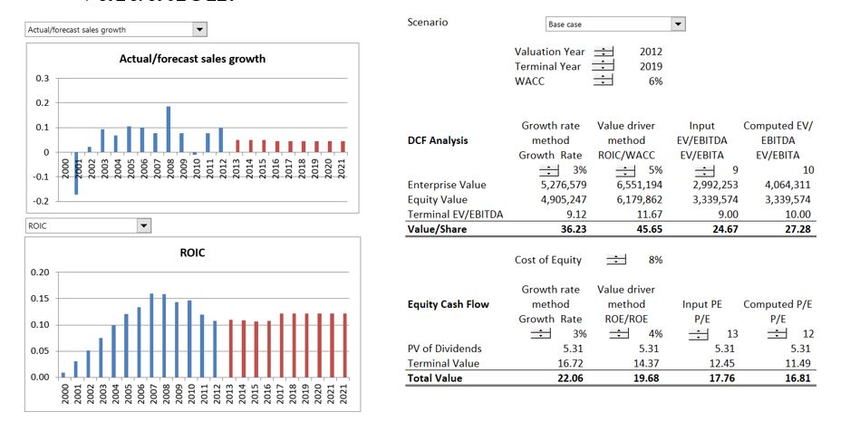
Presenting Key Assumptions with Flexible Graph and Historic Switch
After you have evaluated the returns, you can begin assessing assumptions. I suggest you make a graph using the INDEX function to make flexible graphs with a spinner box as explained in the associated link. I hope that you do not muck up your model with a bunch of different scenarios. Instead you should put the scenarios for key variables like sales growth, margin and capital expenditures in a separate page. The screenshot below illustrates how you could put some of the assumptions with the history and forecast in a graph.
.
.
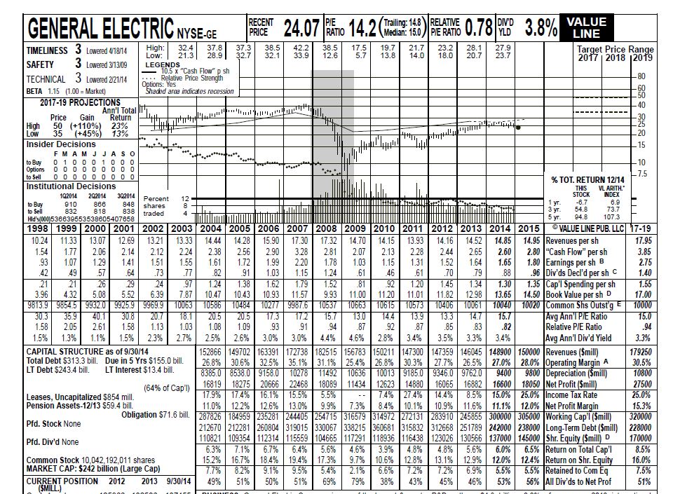
The screenshot below illustrates the idea of presenting history next to assumptions. It is from Value Line and I remember using these summaries in the 1970’s. But the idea of showing all of the long-term history and evaluating the ROE and ROI in the forecast as a test of the assumptions is still very attractive even with all of the stuff you can find on the internet. In the case a hand, the ROE forecast for GE was 15% and the projected stock price from EPS x P/E ratio was projected to range from 50 to 35 with an average 42.5. The actual price
.
.
Implementing Assumptions with Flexible Graph and Historic Switch
When including assumptions in a model you will probably want to make alternative assumptions with respect to certain key assumptions like sales growth, margins (which reflects the price of the product) and capital expenditures (which should be consistent with the sales growth). These assumptions should probably be in a separate page of the model. You can use the INTERPOLATE function to attach assumptions and it is a good idea to use one of the excel forms (spinner or combo box). The screenshot below illustrates how you could implement alternative assumptions in a separate sheet.
.
.
Other assumptions for things like accounts receivable to sales or inventories to cost of goods sold can be based in one way or another from historical data. You can use AVERAGEIF with the historic switch or you can use SUMIF with the last historical year (or the LOOKUP function). In the screenshot below, these assumptions which remain constant are shown in the blue colours. The numbers in red come from the red sheet that includes the different assumptions.
.
.
Section 4: Constructing Your Model in a Structured and Transparent Manner
Once you have created and presented assumptions, you can put the model together. The philosophy of keeping things structured, transparent and flexible is important. Including checks in the model is also a very good idea. As this section will ultimately involve building financial statements, some issues of how to use a model in credit analysis are discussed.
Theory: Separation of finance and operations; depreciation theory and growth (population age and birth rates); evaluating returns with new investment and write-offs; currency adjustments, inflation and McKinsey formula; where to put free cash flow; assessment of forecasts; why balance sheet checks so much of the financial structure; FAST religion; credit analysis and bond rating simulation; cash flow waterfall
Practice: Historic switch and transition between forecasts; timing of models; conditional formatting; setting up debt and cash part; tricky minimum cash analysis with MAX and MIN; key of not starting modelling with financial statements; interpolate and credit score; structuring periodic models.
How can you not begin with operations and free cash flow. How cannot not make the model work in a natural manner. Need to understand required capital investments that are necessary to make EBITDA.
Structure of Corporate Model and Criminal Behaviour in Modelling
All models should have some basic points if they are well structured. There should be a balance sheet and income statement for historic periods at the top. Then there should be an assumptions section that is not messed up with a bunch of scenarios (scenarios should be in a different sheet). Then there should be a section that evaluates free cash flow before tax — the revenues, operating expenses, capital expenditures and working capital changes. After the free cash flow, a depreciation section should be structured that may include some complications if the growth rate or the nature of assets changes. With depreciation (and deferred tax changes and provision changes) you can compute free cash flow. After free cash flow, you should put in a debt and cash section that will be used to reconcile the cash flow with the financial statements. This will give you interest expense, debt balance, debt balance and the required minimum cash. This section can also include other income and other asset balances. With all of these sections, you can finally put together the financial statements. The screenshot below illustrates a very simple model with the various factors.
.
.
There are some things that you should not do in financial models. The screenshot below shows only one example of this where a mixed number suddenly appears in a financial statement and where the financial statements are at the top of the model instead of the bottom of the model. More examples are included in the associated link. Some criminal practices include:
- Hard-coded numbers after inputs
- Forecast Profit and Loss and Balance Sheet at the beginning of the model
- No explicit section that connects the financing with the balance sheet
- No historic switch and method to flexibly move from history to forecast
- Depreciation methods that do not recognize change in net deprecation rate with change in growth rates
- Formulas in the balance sheet
- Meaningless colours that do not provide a guide
- No audit of balance sheet and history
- Polluting the fundamental models with multiple scenarios
.
Adjusting Depreciation for Retirements and Changing Growth
You should know a little growth and depreciation theory. When a population grows slowly, the average person is relatively old (like Japan). This is the same with capital expenditures and depreciation. When you have faster historic growth the depreciation expense is lower relative to net plant. The depreciation divided by the net plant remaining becomes high. When a company is growing fast, the depreciation rate You can find more information on the associated links. The screen shot below shows how you can use the solver add-in in excel to derive at the same time the base level of retirements and the growth rate in retirements for existing assets. These inputs are necessary if you use the gross asset block to forecast depreciation expense.
.
.
Connecting Cash Flow and Balance Sheet and Cash Flow Waterfall
I suppose you could end a financial model at cash flow and evaluate the return on invested capital. You could use the free cash flow in valuation and take the items that form the bridge between equity value and enterprise value from the prior year balance sheet. But if you want to model financing and earnings and net income, you need to incorporate a financing section of your model. The screenshot below illustrates how you could set-up this portion of the model in a case that involves new financing.
.
.
Section 5: Computing Free Cash Flow and Valuation Over Explicit Period and Evaluating the Enterprise to Equity Value Bridge
Theory: Proofs of concepts with models; careful definition of free cash flow with deferred taxes, ; consistency of free cash flow and WACC; EV to equity value and deferred tax; WACC and interest tax shield; political risk and other adjustments to the cost of capital; timing assumptions and 1/2 year assumption.
Practice: Effective Switches and NPV calculations for start and end dates, formula for partial year discounting
Definition and Idea of Free Cash Flow
After creating a financial model and balancing the balance sheet. The first part of this process is evaluating the free cash flow. There are different ways to compute free cash flow. One of the methods is shown below. An example of computing free cash flow is shown in the screenshot below the formula.
- EBITDA
- Less: Capital Expenditures
- Less: Adjustment to EBITDA for changes in working capital
- Add: Other adjustments for warranty provisions
- Add: Changes in deferred taxes
- Less: Operating Taxes without interest – EBIT x Tax
- FREE CASH FLOW
.
Adjustments to Free Cash Flow and Consistency with Enterprise Value to Equity Value Bridge (Net Debt)
There are a number of issues related to making sure the free cash flow items correspond to the final valuation. Take the example of deferred taxes. You could make deferred tax liabilities a subtraction in the net calculation. Alternatively you could compute the change in deferred tax and put them in the free cash flow. For this case and provisions you should include changes in deferred tax and changes in provisions as items of cash flow.
.
.
Evaluating the Return on Investment and Understanding that Returns Fall After New Investments (and Increase After Write-offs)
There is little other way to evaluate the assumptions. You can be sure that you projections are crap when the return increases a lot compared to history.
Section 6: Terminal Value and Multiples
Theory: Terminal value from P/B and ROE; use of value driver and multiples in terminal value; stable and normalised cash flow for terminal value period; consistent and reasonable multiples; value of interest tax shield and APV;
Practice: Conditional formatting for terminal period; using user-defined functions for complex calculations; using terminal value switch; using TRUE/FALSE in present value calculations.
Terminal Value Philosophy
The DCF makes a forecast that in theory is supposed to reach some kind of stable cash flow (as if there is any day in your life that your life is stable and will stay like that). Most of the value should come from the terminal period – this is like buying a stock, holding it for dividends and then selling it. Your final result will be driven by the capital gain. Methods for computing terminal value and deriving stable long-term cash flows are the real issue in applying the DCF, whether for a financial company or for an industrial company. To introduce terminal value, the first step is to evaluate what terminal growth, terminal ROIC and other terminal value assumptions are reasonable.
.

Alternative Terminal Value Methods
- Industrial Company
- Constant growth (1+g)/(WACC-g)
- Terminal EV/EBITDA
- Use of Value Driver (1-g/ROIC)/(WACC-g)
- Financial/Insurance Company
- Constant growth (1+g)/(k-g)
- Use Terminal P/E Ratio with Net Income
- Apply Value Driver (1-g/ROE)/(k-g)
- Use regression: P/B = A + B x ROE
Stable Cash Flow for Terminal Value
An absolute fundamental point about investments (whether they are personal investments in education, gambling investments or investments in research and development) require putting some money into investments in order to gain a return (EBITDA). If you want to grow the EBITDA faster, you need to make more investments. If the EBITDA is growing more slowly, you need less investment.
For working capital changes or for capital expenditures, the same principle applies. When the revenue growth changes, the working capital investment changes. In the case of working capital changes, hte process is fairly simple. You can use the formula:
Stable WC Change =
WC/EBITDA * EBITDA t * terminal growth/(1+terminal growth)
For capital expenditures to depreciation and for deferred taxes and even for changes in provisions, you find stable ratios.

.
Section 7: Converting Corporate Model into Acquisition Model
Theory: Alternative measures of cost and benefit of acquisition; computing npv of synergies after tax and comparing synergies to premium; evaluating multiples with and without tax for EV/EBITDA; earn-outs and options in merger analysis; tax issues in mergers;
Practice: Setting up dates for the transaction; using LOOKUP or INDEX and MATCH to convert models; setting-up sources and uses and pro-forma balance sheet; using terminal value switch; using TRUE/FALSE in present value calculations. A few terms that will be used throughout the course.
Mergers and Acquisitions are valuation and capital budgeting problems, but:
- The value of synergies and management strategy in M&A are difficult to quantify with financial models
- Costs and benefits of a merger can be measured in various different ways (DCF Valuation, Equity IRR, EPS changes, credit quality, NPV)
- Accounting, tax, and regulatory issues can be complex in modeling (goodwill, tax step-ups, re-financing)
- Methods of quantifying the costs and benefits of M&A with financial model
- Merger or consolidation; performance of combined company in terms of EPS and credit quality (as well as DCF of target company)
- Acquisition; model the rate of return earned assuming that the company will be re-sold after a holding period and evaluate EPS effects (as well as DCF of target company)
Section 8: Risk Analysis with Alternative Scenario, Sensitivity, Spider and Waterfall Diagrams
Once you have the acquisition model and the standalone valuation model built, you can create all sorts of different kinds of scenario and sensitivity analysis. The fundamental thing to do in any of the scenario or sensitivity analysis is to create a scenario number and use the INDEX function. This is described in the link that is attached to this sentence using the famous bankers life scenario model. You can then extend the scenario analysis to a sensitivity case with a data table and the TRANSPOSE function. This is demonstrated in the associated link.
.


.
Section 9: Alternative Cost of Capital Techniques for Equity Cost of Capital
Theory: Problems with CAPM — all inputs; problems with DCF techniques; use of market to book ratio as alternative; reasonable cost of capital results; inflation and cost of capital; biases in McKinsey formula with inflation.
Practice: Regression analysis on ROE and market to book ratio; computing beta with different series;
- Theory of inflation: if no growth except for inflation and constant nominal return that includes inflation, then income includes the rate of return with inflation as well as
- P/E = [(ROE-g)/(k-g)] * [(1+inf)/(ROE-inf)]
- This formula gives you the real P/E ratio from nominal inputs.
- Observe P/E ratios that are understated in places with high inflation, because:
- The E and the P are not measured at the same date – the E is a forward number and the P is today’s price. When the E is reduced, the true P/E is higher.
The E does not measure the loss in value from assets that are measured at book value and must be replaced at market value. When the E is adjusted to reflect the increase in value, the observed P/E is less than the corrected P/E.
Synthetic Bond Rating with Corporate Models
There is little other way to evaluate the assumptions. You can be sure that you projections are crap when the return increases a lot compared to history.