This article addresses wind production analysis including models of electricity production from wind, wind resource analysis and wind power variability. Data sources for wind analysis including detailed wind data and a database of power curves are presented and analysed. The discussion begins with general information on wind from websites and wind maps and moves to simulation of power production. Alternative ways to evaluate wind data are presented including techniques to speed up calculation with very large files. Methods to integrate power curves with wind data using the interpolate function are illustrated along with the variation that should be expected from wind analysis. Statistics that measure the variability of both wind and power production are introduced so that you can evaluate the general magnitude of difference in P99 and P50 that you would expect from variation in wind speed alone.
The subsequent page extends the analysis to deal with some tricky wind resource subjects and discussion of the difference between measurements of production using a P90 ten year estimate and a P90 one year (you could substitute P99, P95, P75 etc. for the P90 in the sentence). On this page, some subjects related to wind production variability are introduced including what to generally expect as to the annual variability in winds speeds themselves and what to expect with respect to power production that combines wind speeds with power curves. A central theme of much of the wind resource analysis is that there is a great deal of variation that comes from things other than wind speed variation and that this other variation that often has little explanation drives the sizing of debt and can have a large effect on the equity IRR.
.
.
Power Point Slides Describing Resource Analysis and Financial Analysis of Wind Projects
.
.
.
Updated Excel Files with Power Curves and
.
More Technical Exercises and Discussion of Renewable Resources, Storage and LCOE
The files below have different illustrations of resource analysis primarily using hourly data in PVGIS from the EU. This website includes hourly solar irriadiation as well as hourly data for wind speeds. The files demonstrate how to compute detailed resouce analysis with temperature coefficients and adjustments to wind speed to evaluate the uncertainty of the resource and present the hourly capacity factor.
I have created three excel files that accompany the power point slides and are designed to go with the course. The first file is a long-term analysis that contains solar and wind data from different sights that is obtained from http://re.jrc.ec.europa.eu/pvg_tools/en/tools.htm. With this file you can evaluate hourly, daily, and annual weather data that drives the risk and economic analysis. The second file is a smaller file that contains analysis of one year with details on performance ratio for solar and power curve and wind shear for wind. This file is used to illustrate different risks that arise from technical details. The The files below I compare the costs of alternative technologies. I demonstrate that the Lazard website on LCOE can be boilded down to a few key drivers of cost including the capital cost, the operating expenses, the capacity factor and, importantly, the cost of capital. The file ultimately compares the cost of renewable plus battery with other alternatives.
.
.
.
.
.
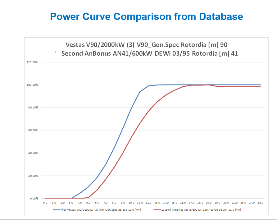
Power Curve Database
Large Excel File with Hour by Hour Wind Data and Simulated Wind Production From Different Wind Farms
Power Curves 2010 in Retscreen.xls
Power Cuves.xls
Acquiring and Analysing Wind Data
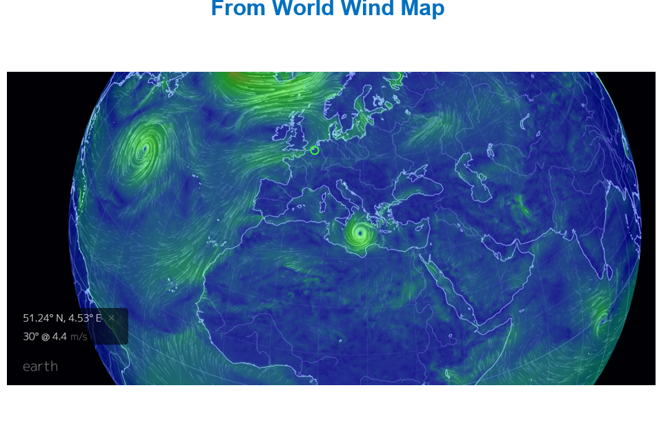
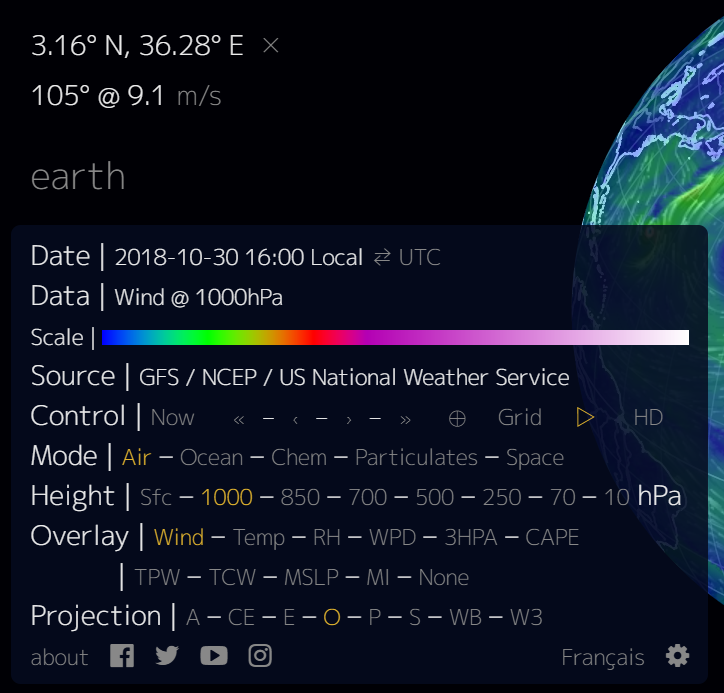
To introduce issues associated with wind resource I like to look at the website from the link below that tracks wind speeds around the world at any instant. You can click on the option for measuring the wind speed into meters per second data and choose on any place in the world to see how fast the wind is blowing. You should see where some of the major areas for on-shore wind production are in the world like Lake Turkana in Kenya, Ireland, south Argentina and the middle of North America. One thing that should also pop out at you is the amount of wind resource off-shore relative to on-shore wind speeds which should make you think about the future of electricity energy as off-shore wind versus nuclear power.
Screenshots below the link illustrate a couple examples of the wind speeds during a particular instant. Note that the place I selected in NL has a wind speed of 4.4 meters/second. The second screen shot shows some of the options you can use with the website including selection of the height at which the wind speed is measured. As discussed a lot below when the wind speed is less than 3-4 meters per second, there will be very little production.
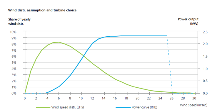
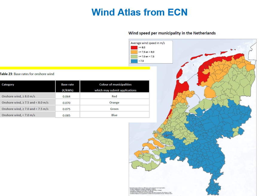
There is of course a vast amount of information you can find on wind speeds and wind maps. For example, if you go the the website for feed-in tariffs in the Netherlands, you will see the wind map that I have put in the screenshot below. Notice how the wind speed is higher near the coast where it is supposed to be more than 8 meters per second. The problem with analysis of wind resources is that wind speeds tend to be very location specific and depend on local terrain among other things. This means that detailed wind studies at a proposed site are necessary and wind measurement cannot come from a simple map like the one shown below. As I discuss later in this page, the amount of wind production coming from a turbine also depends on the distribution of wind. If the wind speed was for example 8 meters per second every hour, the production would be very different than if the wind speed was 6 meters per second for half of the year and 10 meters per second for the other half. This is because the power curve that measures wind production for a given wind speed is not a 45 degree straight line like it is for solar.
Analysis of Hour-by-hour Wind Data
The first detailed subject I address on this page is what does the wind speed data look like and what kind of variation is there from year to year in wind speeds. Finance people care most about annual wind data because debt repayment is not made on a day by day basis but on a semi-annual basis. It is cash flow variation over a longer period like a year that drives risk (I suppose that you could argue that they care about semi-annual wind speed variation because debt service is typically made on a semi-annual basis). So lets see where you can find the detailed hourly data and how you can analyse the risks associated with wind resource. Once the wind data is evaluated, power curves that convert wind data to electric power is addressed and the variation in power due to wind variation is quantified.
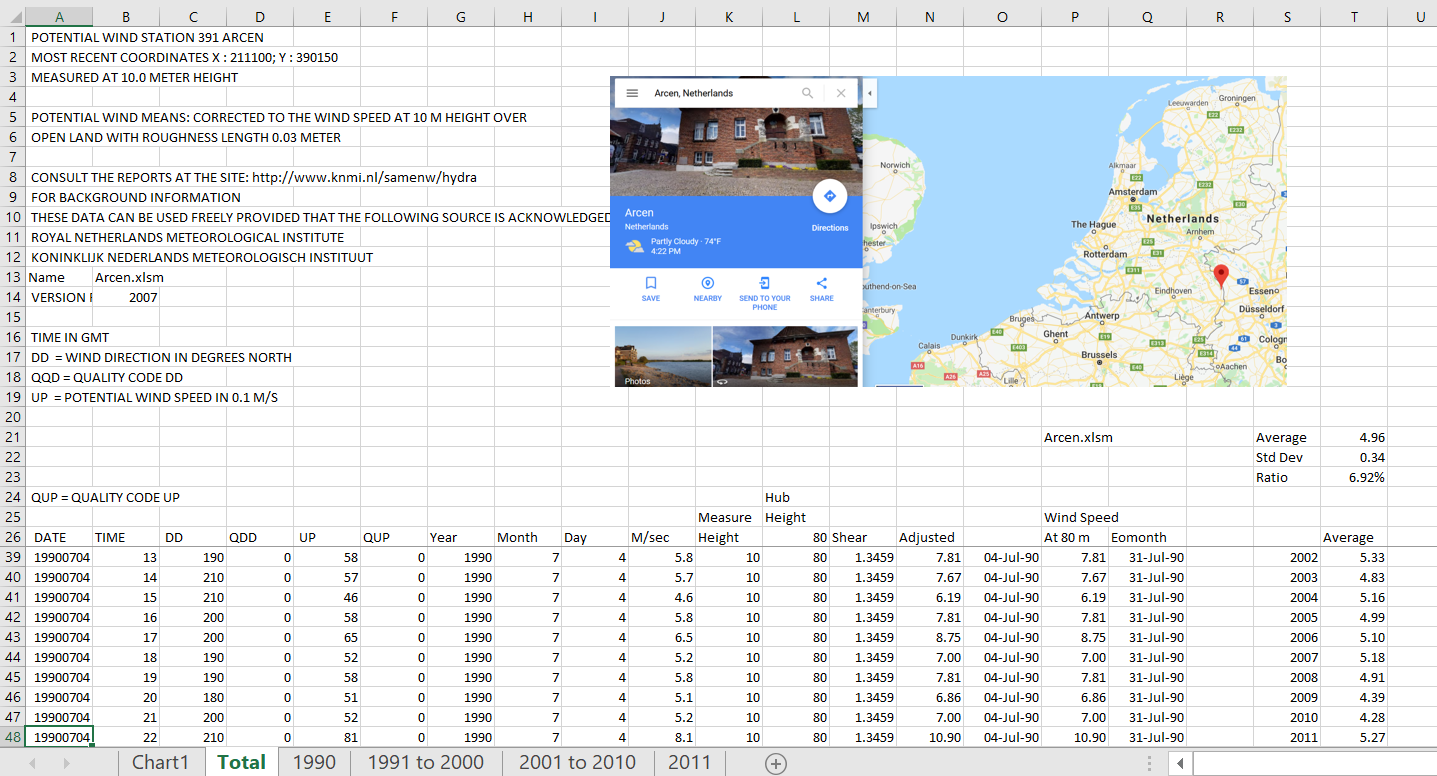
As I sometimes teach in Amsterdam, I have made a case study with Dutch wind data. The good news is that a couple of years ago I found hour by hour wind data for many areas in the Netherlands (NL). (I cannot seem to find it now). With this hour by hour data you can do a lot of stuff. The hour by hour data and the website where I found the data is illustrated in the screenshot below. There is a whole lot of data in these wind files and the difference between wind speeds in different areas is dramatic. The files that you can download below have the hour by hour wind speed data for many years. You can download excel files with hourly wind speeds using the buttons below. I do have other wind data in the resource library but I have not bothered yet uploading the data. If you send me an e-mail to edwardbodmer@gmail.com you can get the other wind speed data.
Excel File that Goes to NCOAA Data and Retrieves Hourly Wind Speeds for up to 30 Historic Years
Excel File with Examination of German Wind Speeds and Question of Whether Wind Speed is Declining
File with Documentation of Methods for Collecting Wind Data and Website Source for NCOAA
Each of the files is set-up with a format illustrated in the screenshot below where there are up to 8760 x 20 rows of data. The raw data shown in the screenshot is adjusted for the wind shear factor as explained in the next section. After the raw data shown in the screenshot is adjusted for the height of the turbine, I demonstrate how you can very easily compute annual wind speeds using the SUMIF function. You can also evaluate the distribution within a year and see that within a year wind does not follow a normal distribution. This is due to the simple fact that wind speeds cannot be negative.
Wind Shear Factor and Turbine Height
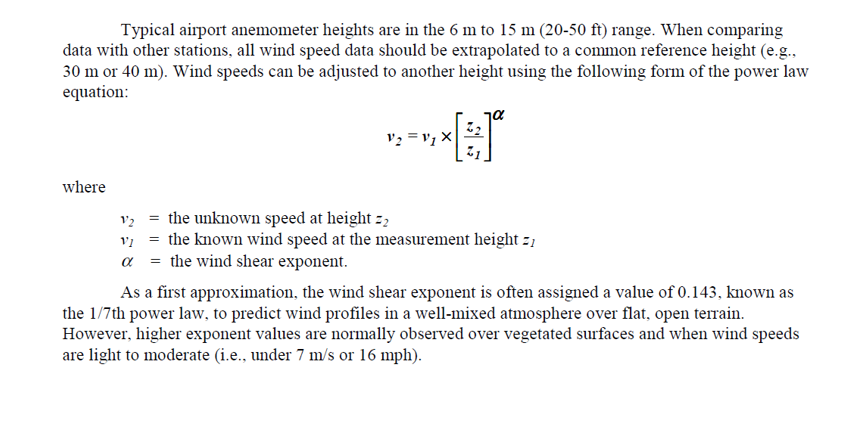
Wind speeds are more at higher heights (until you get out of the atmosphere). If the hub of the wind turbine is at 100 meters but you are measuring wind speed at 10 meters, you need to increase the wind speed. The difference between wind speed at 10 meters and 100 meters is called the wind shear. To compute the wind shear when the wind speeds are measured at a different height than the hub height of the turbine, a power coefficient of 1/7 is often used. With this power coefficient, you then raise the ratio of the hub height to the measured height by that factor. The wind shear is discussed in the screenshot below.
The wind shear formula works as follows. First divide the hub height by the measured height (e.g. 80/10) to the power of the shear factor: (80/10)^(1/7). This gives you an number that is greater than 1.0. Then, multiply that result by the wind speed measured at 10 meters. For 10 meters versus 80 meters and a power coefficient of 1/7, the multiplier for wind speeds is 1.3459 as shown in the screenshot above.
Annual Variation in Wind Speeds, P99 and SUMIF
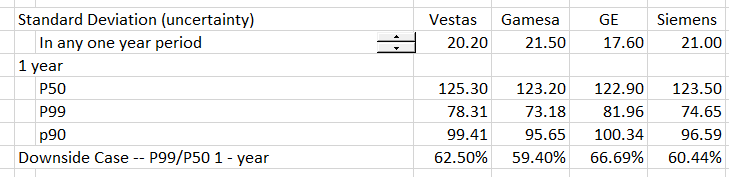
In some wind studies I have seen the difference between the P99 worst case and the P50 base case for as much as 60%. (For now think of the worst single year in 100 years or a one in one hundred year event for wind). The question addressed in this section and the next section is how much variation comes from pure wind speed variation. In the next page you will see that much of the P99 variation comes from modelling errors that can be measured on a relatively arbitrary basis. To introduce the issue of how much variation comes from variation in wind speeds the screenshot below illustrates a case where the downside case (1-year P99) is 60% worse than the P50 case.
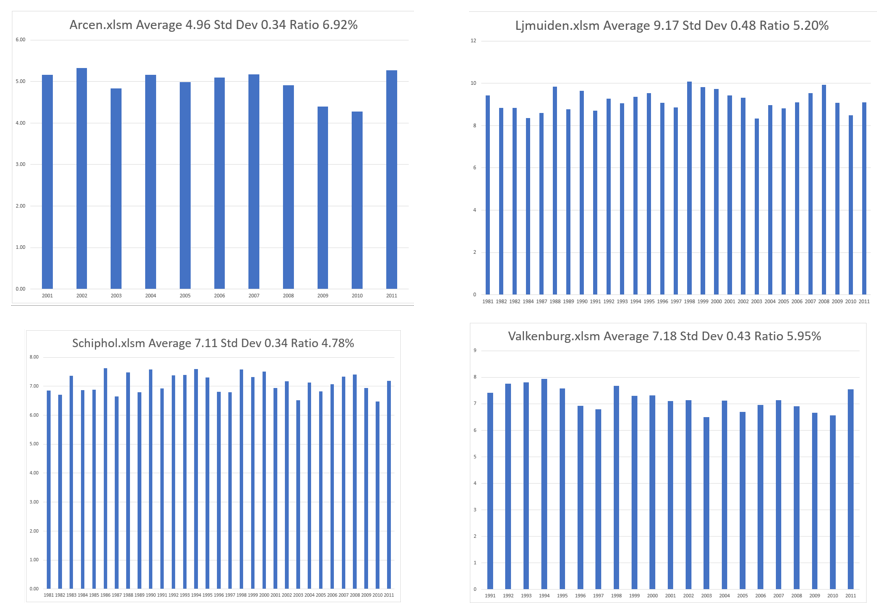
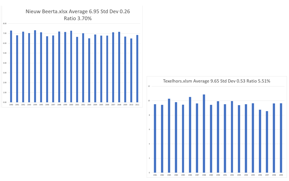
The first step in evaluating the wind speed uncertainty is understand how much downside comes from pure year-to-year variation in wind speeds. The examples below show that annual variation in wind speeds ranges from 3.7% to 6.9%.
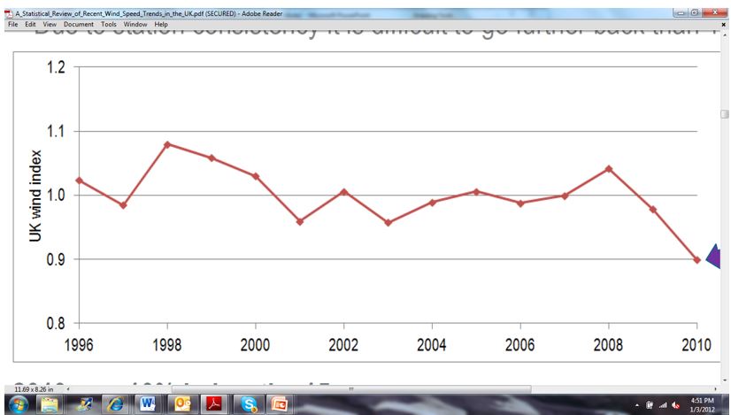
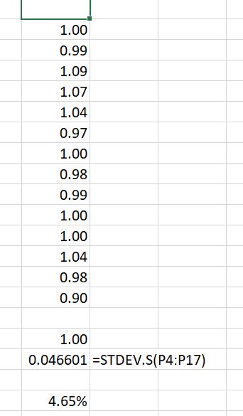
Another example of wind variation comes from a presentation made about a low wind year in Britain. Note the last number that was 90% of the index value in 2010. While this seems very low, the standard deviation relative to the average over the 15 year period was 4.67% which is about the level shown for the Dutch wind. You can use the NORMDIST value with an x-value of .9, a mean of 1.0 and a standard deviation of 4.65% and see that the probability is 1.58%. This is like the P values discussed later on.
.
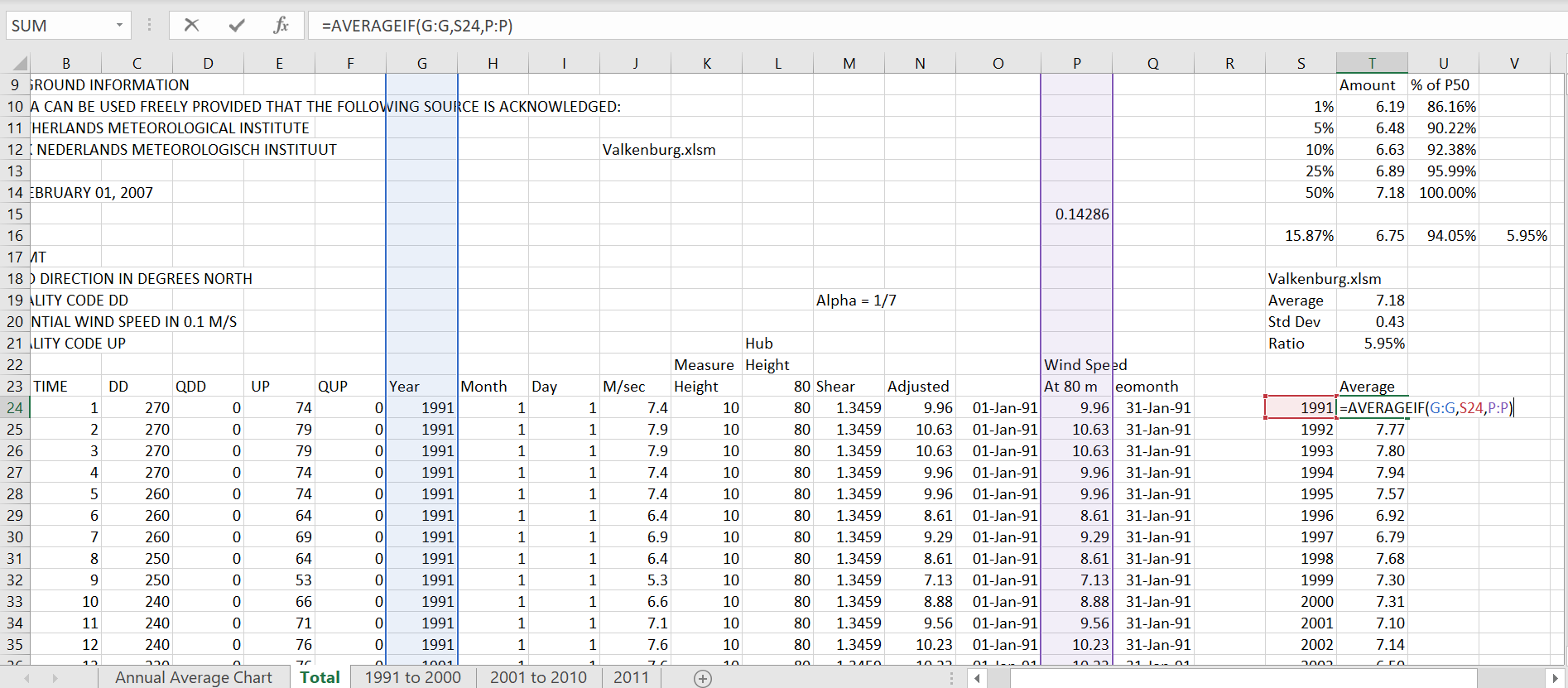
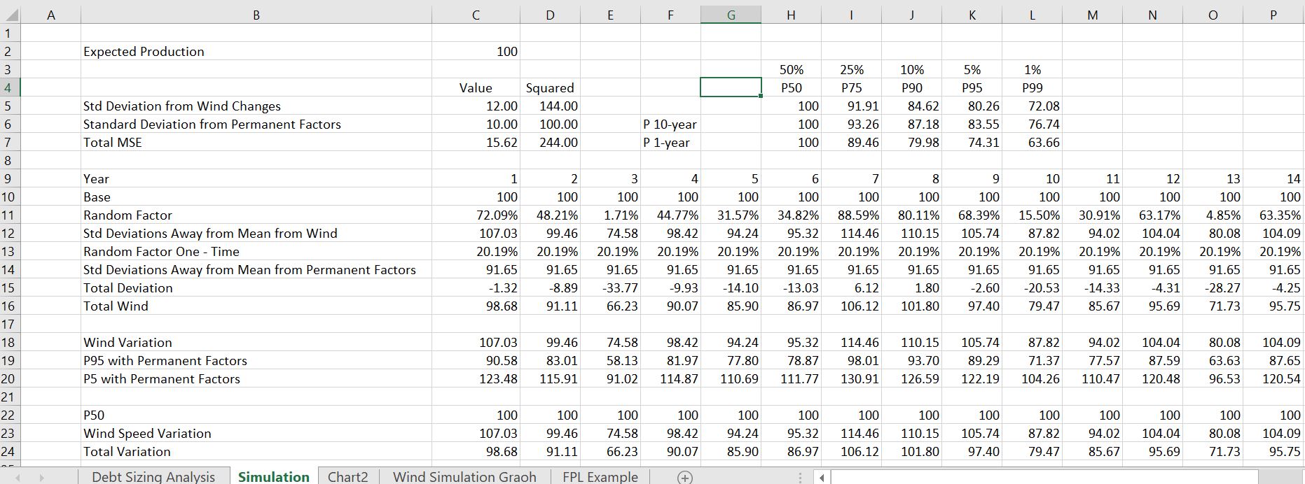
The calculation of annual wind speed variation from hourly wind speeds is very simple. You just make a column with the years and another little table with the years. Then you use the AVERAGEIF function next to the little table and you use the entire columns. This is illustrated in the screenshot below where you can see the table at the right of the page. Note that entire column G for the detailed year is the first input and you don’t need to press any F4 key. The final input, column P is for the individual hourly wind speed.
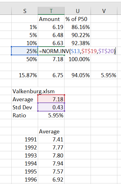
At the top right of the of the above screenshot, the implied P99, P95, P90 and P75 are computed from the wind speeds. This comes from the assumption that the distribution of annual wind speeds is normal. If you have the average and the standard deviation, the P99, P95, P90 and P75 are very easy to compute. All you have to do is use the NORMINV function as shown in the screenshot below. For the P99 case, you use a 1% probability and the mean and the standard deviation. The implied one in 100 year wind speed from the NORMINV function is 6.19 relative to an average wind speed of 7.18. This case is for an area that has relatively high variation in wind speeds. The major conclusion from this analysis is that the P99 case reduces the wind production by about 14% and it is 86% of the base case. I also present the tail of one standard deviation with the 15.87% case (1-68%)/2. In this case the standard deviation divided by the average is one minus the percent reduction.
Before moving to how the distribution in wind speeds translates into distribution of wind production I discuss how you can evaluate the distribution of wind speeds within a year. The distribution of wind speeds is important because the power curve is not a straight line with 45 degrees. To compute the distribution you can follow the following steps:
- Use the EIS to make a column of 8760 rows
- Input the year you want to evaluate
- Use the MATCH function with the year you input and the column with the year for each hour
- Next to the 8760 rows, add the result of the MATCH function to the number
- Use the INDEX function to fetch the appropriate number from the hour by hour data
- Create a list of wind speeds (e.g. 0 to . to 1.0 to 1.5 etc.) and use the FREQUENCY distribution to accumulate the number of observations for each wind speed. Then divide each increment by the sum of observations to derive the probability distribution.
- Use the NORMDIST function without the cumulative option and with the average and standard deviation to compute the probability of different wind speeds assuming a normal distribution.
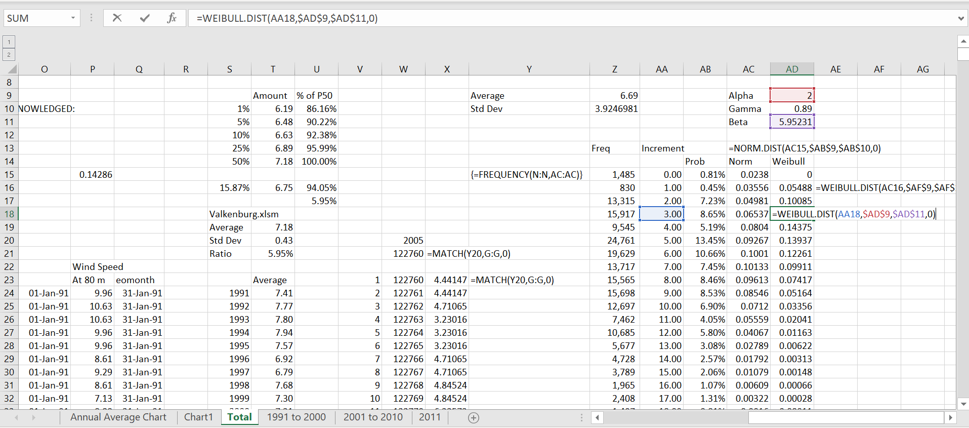
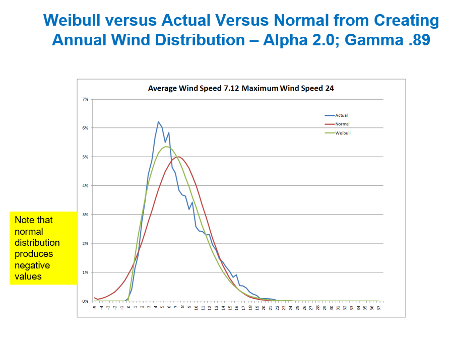
- Use the WEIBULL function with an Alpha of 2.0 and an Beta of .89 x the average wind speed to compute the skewed weibull distribution in the same manner as the normal distribution.
The computation of distribution of wind speeds is shown in the screenshot below. I have put some of the formulas described above next to the cells. When you use the NORMDIST or the WEIBULL functions you have to be careful that the distribution adds up to 1.0 (if you use increments of .5, then you should divide the distribution by 2. This case below uses the year 2005 which begins in row 122760.
The graph below shows a case where I show the distribution of actual wind speeds compared with the simulated wind distribution from normal and Weibull distributions. Note how the normal distribution predicts that there will be negative wind speeds. I have tried this with other wind distributions and the alpha and gamma shown in the graph below do not work nearly as well. In the end, it may be best just to use the actual distributions instead of trying to take short-cuts with distributions.
Putting Together Wind Data with Power Curves to Derive Wind Production
In this section I convert the wind speed data to wind production data. The manner in which this is really done is shown in the table below where the analysis includes various losses as well as the power that comes from the wind. The manner in which wind production can be converted to electricity production is illustrated in the screenshot below.
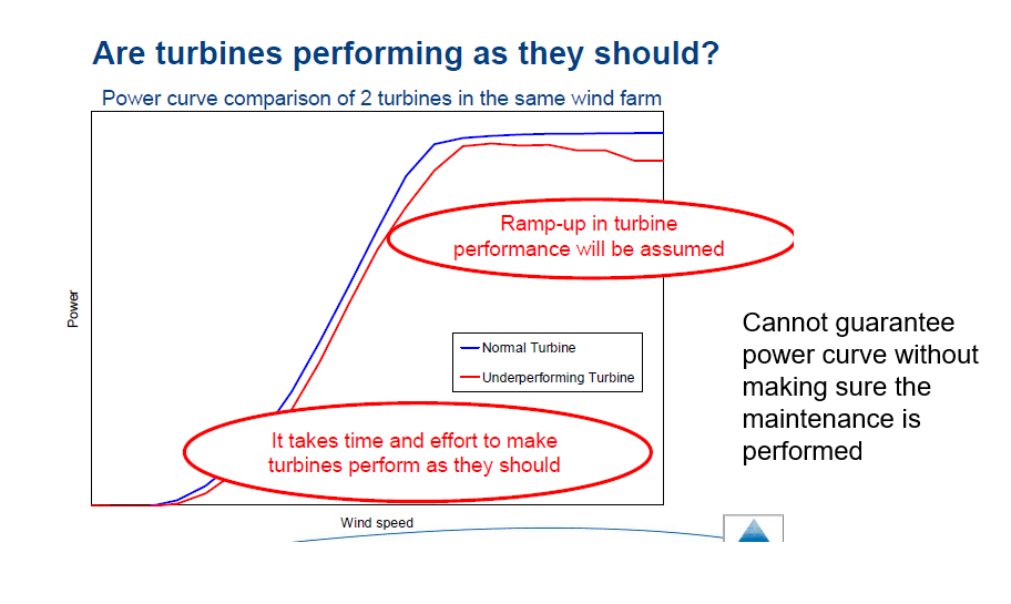
Power curves translate wind speed into power. They are perhaps the most crucial element in understanding wind power. You can sometimes guarantee the power curve.
Wind Analysis and Power Point Slides
General ideas of measuring wind speeds, wind power, power curves and variation in wind are explained in the slides that you can download below. The slides also use the Netherlands feed-in tariff as a case study and use the perspective of credit analysis from the perspective of a bank. You can get the slides by clicking on the button and downloading the file. As with the discussion below, the slides begin with speed analysis (no electric power or turbine). Then the turbines are added using a power curve to convert the wind into electricity and the power curve database is introduced. Finally actual wind production variation from year to year is evaluated.
Files associated with Lesson Set 1: Wind Resource Analysis
In this section I describe how to compute the P90, P99 etc. from power curves and historic wind data. This involves compiling hourly wind data and matching the wind data against power curves. In addition, actual wind variation is evaluated for a number of wind farms using the Generation Database below. Computing the P90 or P99 etc. can be derived from hourly wind data and power curves. You can use the LOOKUP function to evaluate the amount of power at different wind speeds and the NORINV function to evaluate probability distributions. The hourly distribution of wind can also be computed from a Wiebull function as illustrated in one of the files below.
File with Analysis of P50 and P90 with Monte Carlo Simulation and Mean Square Error Evaluation
The file below demonstrates the credit analysis of a wind farm from a long time ago. It demonstrates how the P90 and P95 can be used in assessing the credit analysis of a wind farm with downside analysis. As this write-up has multiple wind farms, it can be used to compare capacity factors and other factors for different wind farms.
S&P Credit Analysis of Multiple Wind Farm Describing Risks including Wind Resource Risk with P95
.
.
.
Excel File with Hourly Detail that Includes Temprature Coefficient, Performance Ratio and Wind
.
.
Wind Playlist
There are a series of videos that describe the various issues associated with analysing wind projects. I have no idea how you could watch all of these videos without going crazy. But you may want to tak a look at a couple of them. I have included a button with a link to the LCOE calculator.
If you want the files associated with wind I have the files in a folder (chapter 1, project finance/featured models/wind) of the resources. Just drop and email to edwardbodmer.com and I will send a google drive with a whole lot of stuff (probably too much). But you can unzip the files and look for what you want and save the google drive in the cloud….