Use of Proofs in Corporate Valuation Analysis

When working through corporate finance and valuation issues, it is often the case you may get into debates about various issues.  Examples may be treatment of non-paid employee reserves, deferred taxes, fair value of derivatives, WACC issues related to tax shield, target capital structure, surplus cash, the timing of the value driver formula.  When debating various concepts, you can use a model to prove the various ideas and resolve debates.  These proofs generally involve the following in corporate finance:

1. Make a long-term model with the NPV function to prove the true value

2. Create a model that uses the technique that is being debated

3. Demonstrate that the valuation model you have created conforms to the long-run model.

 

Example with Terminal Value and Value Driver Formula

I received the following question:

I noticed for terminal value you are calculating off of the FCF based on the final year of explicit forecast instead of the year after. I know with the value driver formula where NOPLAT is used, you are supposed to calculate the NOPLAT in the next year, but use the discount factor that is same as the final year of explicit.

 

The basic answer to the question is that you should use (1+g) anytime you are applying a cash flow in a terminal period to compute value.  This is just due to calculus and integrating cash flows from the next period to infinity. So, in general you could either use the terminal year cash flow x (1+g) or the next year cash flow. But it is true there are complications with the value driver formula that I have maligned on many occasions in this website.

If you are going to use the value driver formula V = NOPAT x (1-g/ROIC)/(WACC-g), then, if the growth rate for the terminal period is not the same as the historic growth rate, the (1+g) you should use is the historic growth in the terminal year investment and not the prospective terminal growth.  This is because the prior year growth drives the investment base and then the growth continues at the terminal growth rate.  This means you can use one of the following two formulas for terminal value:

1. Value = NOPAT in Terminal Year x (1+Historic Growth) x (1-terminal growth/ROIC)/(WACC-g)
2. Value = NOPAT in Terminal Year + 1  x (1-terminal growth/ROIC)/(WACC-g)

The real problem with the value driver formula comes when there is a change in the assumed return from the historic return. In this case the whole value driver formula falls apart. To demonstrate why these formulas work and why the formula falls apart, you can work through a proof.

If you assume the terminal value derived from a stable value of cash flows that will grow at different rates, you can use (1+g) applied to the terminal cash flow.

 

The question is interesting and highlights various issues in the mathematics of corporate finance:

1. Because of integrating a number to infinity, you should always use the prospective cash flow in a formula when you divide by cost of capital minus growth.  For example, the classic dividend growth model is V0 = D1/(k-g), but with constant growth, this can be expressed as V0 = D0 x (1+g)/(k-g).  This is fundamental and does not have be be demonstrated.
2. Use of the next period means in any formula that uses k-g in the denominator with constant growth in cash flow, the future cash flow should be used.  If you are in the terminal period, the value driver formula can be BV t x ROIC x (1-g/ROIC)/(WACC-g) or, if there is no change in ROIC, you could put (1+g) into the formula and use NOPAT x (1+g) x (1-g/ROIC)/(WACC-g).  You could also use, as the question suggested the subsequent year NOPAT.

Setting-up a good proof can be tricky.  For the first case I use the same growth rate, return and cost of capital over time with no terminal growth or return differences.  Setting-up a model that computes value with a dividend/ROE method and an free cash flow/ROIC method is demonstrated.  I assume no taxes and no debt so that the two models produce the same result in terms of cash flow and value.  With a long-term analysis I use the NPV formula to compute value in both cases.

Before discussing the model, review how easy it is to derive the value driver formula under constant growth, return and cost of capital:

Value = Dividends 1 /(cost of capital-g)

Dividend 1 = Earnings 1 x  Payout

growth = ROE x (1-Payout) or Payout = 1 – growth/ROE

Value = Earnings 1 x (1-growth/ROE)/(Cost of capital-g)

Step 1: Set-up Timeline with Theoretical Long-term Cash Flow and Terminal Value Time Line

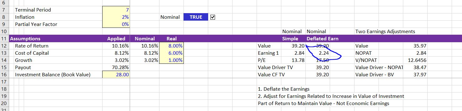
The first part of the proof shown in the screenshot proves this formula which can, under constant growth be expressed as Value = Earnings 0 x (1+g) * (1-g/Return)/(Cost of capital – g).  To set the model up, enter the assumptions and a time line.  Use ALT, E, I, S to quickly make a 1000 year model.  Open the generic macros file to colour the sheet.  The assumptions and a set-up of a time line with TRUE and FALSE is shown in the screenshot below.  Note that there are switches for the explicit period, the terminal date and the period after the terminal date.

 

 

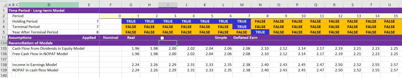
To evaluate alternative terminal value calculations you can create and investment balance; the book value of equity or the book value per share. For these problems it is almost always appropriate to assume that can flows occur at the end of the period consistent with the assumption in the NPV and IRR formulas.  This means that to compute returns and interest you should use the opening balance.  As the ROI = Income/Investment, you can compute income as the opening investment balance multiplied by the ROI.  Dividends can be derived from the dividend payout ratio multiplied by the income where the dividend payout ratio is  a function of return and growth: DPO = (1-g/ROE).

The screenshot below illustrates the long-term model (the year 1000 is shown at the right). The present value of dividends are 39.20. (The half year convention where cash flows are moved up to the middle of the year through multiplying by (1+cost of capital) ^ .5).  This is the base for testing other methods.

The screenshot below shows the value of the company using the NPV formula.  The NPV of dividends over a long period of time produces the theoretical value of the company that should be the same when other methods are used that do not extend to the entire long-term period.

 

 

Step 2: Testing Alternative Terminal Value Formulas to Make Sure they Produce the Same Result as the Theoretical Cash Flow Approach

 

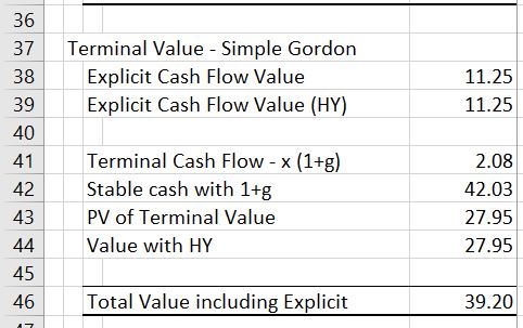
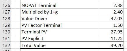
The excerpt below shows results of valuation when applying the terminal value in the constant growth scenario.  In this excerpt, the explicit cash flow from year 1 to year 7 has a value of 11.25.  The terminal year cash flow in period 7 is 2.08.  When this value is multiplied by (1+g) and the value is computed, 2.08 x (1+g)/(k-g) is 42.03. This value is discounted based on the value to year 7.  When the 11.25 explicit value of cash flow is added to the value of 27.95 the total value is 39.20.

 

 

The screenshot below shows results when the value driver formula using the formula:

Value = Closing investment balance x ROE x  (1-g/ROE)/(k-g).

This is equivalent to Value = Income x (1-g/ROE)/(k-g), because Income = Closing investment balance x ROE. The closing value of the investment in year 7 is 30.02.  But using the closing value of the investment.

 

 

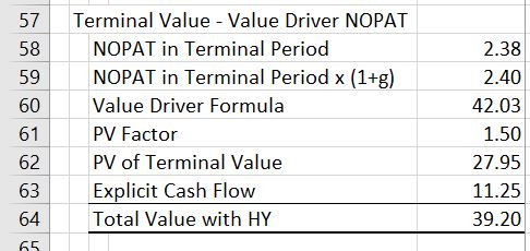
The summary below demonstrates how the value driver formula works with equity flows where there is a constant growth rate. The NOPAT is the income in the terminal year from the above screenshot that lays out the investment balance.  When this NOPAT is multiplied by (1+g), the NOPAT from the year after the terminal period is derived and the valuation using Value = NOPAT x (1+g) x (1-g/ROIC)/(WACC-g) produces the correct number.

 

 

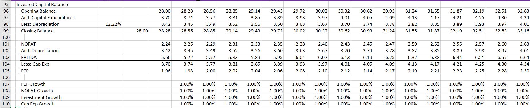
Investment balance to compute the stable ratios that are needed for the free cash flow model. Need net plant depreciation rate and the accumulated depreciation. Note that you could use a UDF for this.

 

 

 

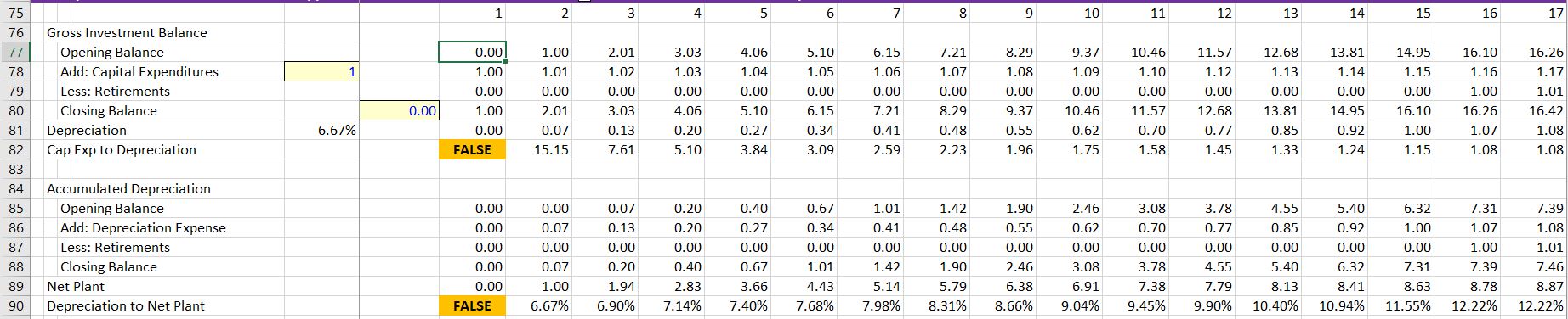
Conversion to Free cash flow model.  Compute invested capital balance and use the stable depreciation and stable capital expenditure.  Show the growth in various factors.

 

 

Case with ending book value.  Can use instead of NOPAT.

 

 

 

Case with Terminal Value and constant growth.  Can use (1+g).  Problem later when changing growth and changing return.  Se how to use LOOKUP or SUMIF to find the number.

 

 

Inflation Adjustment and P/E or EV/EBITDA ratios

What does it really mean

 

 

 

 

 

 

Application of WACC in the DCF

Video explanations include theory and some background APV does not add anything new to valuation. Correct application of the WACC accounts for all items in the bridge between equity value and enterprise value in the WACC calculation. Investment bankers typically do this with using net debt rather than gross debt in computing WACC. Similar adjustments to the WACC should be made for associated investments not included in EBITDA, the fair value of derivatives, discounted operations and any other items.

 

 

Cost of Capital Subject		File Reference		Video Link
Interest Tax Shield Part 1 with Introduction to Net of Tax Method		Interest Shield Exercise		https://www.youtube.com/watch?v=G6BBvAFHJGo
Demonstrate that Net of Tax Method in Capital Structure Values Tax Shield		Interest Shield Exercise		https://www.youtube.com/watch?v=9LKppeYudVU
How to Compute Ku with Net of Tax Method		Un-lever and Re-lever with Tax Shield		https://www.youtube.com/watch?v=jaLOx3RJFkc
Overview of How Debt Beta Influences WACC		Theory of Debt Beta and WACC		https://www.youtube.com/watch?v=n_csEtMHveA
Demonstrates use of Interpolate Function		Mechanics of Debt Beta and WACC		https://www.youtube.com/watch?v=Bvp0ruVYBSw
How to Compute Ku with Net of Tax and Debt Beta		Unlever and Re-lever with Varying WACC		https://www.youtube.com/watch?v=7ny67y-EpR8
Demonstrates Valuation with WACC and Net of Tax Method		Growth Rate, Tax Shields and WACC		https://www.youtube.com/watch?v=oKNmQ9fimZc
Shows Bias in WACC from Growth		Circularity, WACC and Ku		https://www.youtube.com/watch?v=2EPd8_yi_0M
Shows how to Use Goal Seek to Resolve Bias		WACC Growth and Goal Seek		https://www.youtube.com/watch?v=JEahjlc8QFs
Demonstrates that Target Capital Structure is Irrelveant without Tax Shield		Target Capital Structure without Taxes		https://www.youtube.com/watch?v=1k8Ij-biv3w
How to Resolve Target Capital Structure with Tax Shield		Target Capital Structure with Tax Shield		https://www.youtube.com/watch?v=PkIsIOtAqy4
…………………………………………………………………………………………………………………………….	…	…………………………………………………………….	…	…………………………………………………………………………………………

Application of WACC in the DCF

The files associated with the videos demonstrate how to make appropriate adjustments to the DCF model. For this lesson I did not include exercises as part of the individual files. Instead, if you want credit for completing the lesson set, you should fix the Disney case study that is part of the case study page. Alternatively, you can go to the corporate model page and fix the DCF page in the various models. You should include a page where you find betas and correctly compute the all equity and debt betas using the net of tax capital structure. You should then compute the value of the company using the net of tax capital structure and subtract the net of tax debt. All you have to do then is to send me 40 Euro and you will get your name on the success page. If you have ever taken one of my courses in person, you do not have to pay the fee.

If you are like me, when you study how to apply the WACC in a DCF model you can be frustrated. When you read about applying the WACC in financial articles written by academics with dense equations and esoteric theory your confusion will without question increase. Some articles suggest that you must use APV and discounting tax shields at the all-equity cost of capital. Most write down a seemingly sophisticated formula for Be and Bu as a function of Bd and the tax rate. This lesson set addresses many of the issues including application of a target capital structure, un-levering and re-levering beta, resolving an apparent circularity problem and valuing the tax shields created by interest. The video below introduces some of the issues.

I have tried to demonstrate that these WACC issues are really not very difficult and do not require a whole bunch of seemingly complex formulas that seem to come from nowhere. Instead I use a couple of simple and hopefully clear-headed ideas along with simple excel models to prove the ideas. Rather than working through the technical formulas without much real explanation, the files and videos in this section demonstrate how to prove a few key concepts. The models are simple financial models. Construction of the models is demonstrated in videos. Key conclusions of the financial model proofs and the theory that I hope is explained in simple terms include:

1. Tax Shields from Interest Deductibility in WACC Can Be Resolved with Gross and Net Capital Structures. The excessive discussion about how to value tax shields associated with debt is a colossal waste of time. When you recognize that the tax shield is equivalent to a reduction in the coupon rate on debt, the proof of how to treat the tax shield becomes clear. The market value of debt to the corporation is reduced to when the coupon rate falls and the equity value increases. For example if debt was 1,000 at with an interest rate of 10% and the coupon rate is reduced to 6%, the market value of debt decreases form 1,000 to 600. If the opportunity cost of debt for providers of funds is 10% both before and after the coupon rate decrease, the value of the debt declines to 60 of interest/10% or 600. This example is just the same as the tax effects of the interest shield at a 40% tax rate. Using the simple an basic principles that the fixed cost to the corporation is reduced from the tax shield and that the opportunity cost to providers of debt does not change from the corporate tax rate, the following equations quantify the tax shield. The second method is equivalent to the traditional WACC implementation.

Tax Shield Percent = Gross Observed Market Debt to Capital * t

Net Equity Percent = Gross Equity Observed/(1-Tax Shield Percent)
Net Debt Percent = 1- Net Debt Percent
Ku = Kd * Net Debt Percent + Ke * Net Equity Percent

Ke = [Ku – Kd * Net Debt Percent]/Net Equity Percent

Bu = Bd * Net Debt Percent + Be * Net Equity Percent

Be = [Bu – Bd * Net Debt Percent]/Net Equity Percent

2. Beta on Debt Should be Derived from Bond Yields: The beta on debt is generally assumed away in considering the WACC. But the debt beta can be derived from the credit spread on debt given the EMRP and Rf. For example, the historic spread on BBB bonds is about 2% and the gearing of BBB companies is about 55%. This implies the beta on debt or Bd is given by the equation Cd = Rf + EMRP x Bd. Restating the equation implies that CSd = EMRP x Bd and Bd = CSd/EMRP. If the credit spread is 2% and the EMRP is 4%, the the Bd is .5. Data on the relationship between debt to capital and credit ratings can be used to derive the beta on debt as a function of the market capital structure

Total Interest Rate = Rf + Credit Spread
Total Interest Rate = Rf + EMRP * Debt Beta
Credit Spread = EMRP * Debt Beta
Debt Beta = Credit Spread/EMRP
Net Debt Percent = 1- Net Debt Percent

3. Bd Should Vary with the Capital Structure in Computing Be and Bu. Even though this is obvious, it is virtually never done in practice. S&P standards for the leverage and credit rating and published credit spreads can be used to establish Bd that varies with capital structure. When the varying credit spreads are applied, the effects on the relationship between Be and Ke and the capital structure are dramatic. The cost of equity at high leverage is dramatically reduced which reflects the call option premium that is inherent in the Ke and the put option cost that is part of the Kd.

Bu = Bd * Net Debt Percent + Be * Net Equity Percent, where Bd is a function of Gross Debt/Capital
Be = [Bu – Bd * Net Debt Percent]/Net Equity Percent, where Bd is a function of Gross Debt/Capital

4. Circularity in WACC and Valuation from Tax Shield can Easily be Avoided. As the equity to capital ratio is computed using the market value of equity and, in turn, the market value of equity requires a value of WACC that is in turn driven in part by the equity to capital ratio. This implies a circular reference seems to exist. This is not much of a problem when the Bu and Ku is established from a comparison set of companies. The remaining circular reference from re-levering the beta can be easily resolved.

5. Target versus Actual Capital Structure Does Not Matter With No Interest Tax Shield. If there is no tax shield, the WACC should not change if you use different capital structure assumptions because the cost of equity changes to compensate for risk created by gearing. This means that without taxes, use of a target capital structure in the context of DCF is not beneficial, necessary or relevant in terms of accuracy or theory. Without the interest tax shield, when the cost of equity is derived from re-levering the unlevered beta using the market value of debt at the valuation date, the result is exactly the same as if the company moves to a target capital structure.

6. APV does not add anything new to valuation. Correct application of the WACC accounts for all items in the bridge between equity value and enterprise value in the WACC calculation. Investment bankers typically do this with using net debt rather than gross debt in computing WACC. Similar adjustments to the WACC should be made for associated investments not included in EBITDA, the fair value of derivatives, discounted operations and any other items.