.
This page explains how to evaluate the probability of achieving different levels of wind production that I refer to as P90, P99 etc. I also address the painful issue of the difference between a one-year P90 and a ten-year P90. At the end of the web page I describe how you can create financial models of tariffs and financing in the context of P50, P90, P99 etc. Measuring the probability of achieving electricity production from a wind project is central debt sizing of a wind project and the measurements are prepared before the financial close of a project. I demonstrate that the P90 or P99 often drive the level of debt. In describing P90, P99 etc. for the one-year case and the long-term case, I begin by reviewing some wind studies and describing two classes of uncertainty that drive the probability analysis. The first source of uncertainty is the variation in wind from year to year with the resulting energy production. The second is modelling error related to quantification of the production before the facility is operational. This second source of uncertainty related to modelling error is a lot more difficult to understand and define. With different sources of variation, I explain how to combine standard deviations (often called uncertainty) with one another using mean squared error. Once the mean squared error is defined the one-year and the ten-year (or twenty-year) P90 and P99 is established. At the bottom of this page I discuss incorporating the P90 and P50 in a financial model where the tariff may be derived from a target IRR on the P50 case and the financing could be derived from either a P50 or a P99 or a P90 case and the financing could further be derived from either debt to capital or from DSCR.
The tricky part of the P90, P99 etc. is to understand the sources of variation in wind production estimates that are mean reverting and that are related to modelling errors that do not self-correct. The first part of this webpage reviews general also describes general issues with performance of wind studies and debt terms related to probability levels of wind. The second section demonstrates some studies of 1-year and 10-year P50 and P90 wind studies and how to use the NORMINV function and the mean square error statistics. The discussion on this web page builds from the prior web page that dealt with variation in electricity production arising from variation in year to year wind speeds that are described on the prior webpage. The additional sources of variation that come from factors such as modelling error, turbulence, wake measurement error, correlation with reference data, availability, environmental issues and other factors are demonstrated. This page explains how to put sources of variation together and evaluate wind reports. Power point slides that explain these concepts are in the file available for download below (these slides are the same as the slides for the previous page). A similar discussion can be found for solar power in the associated link to this sentence. Below the power point file button, I have included two files with financial models that evaluate debt sizing from alternative wind probabilities and the maximum debt to capital. The second file available for download includes the parallel model concept to resolve circular references. Videos that describe these files are below the buttons.
[wonderplugin_video iframe=”https://www.youtube.com/watch?v=9dsgXkQzlas” videowidth=600 videoheight=400 keepaspectratio=1 videocss=”position:relative;display:block;background-color:#000;overflow:hidden;max-width:100%;margin:0 auto;” playbutton=”http://edbodmer.com/wp-content/plugins/wonderplugin-video-embed/engine/playvideo-64-64-0.png”]
[wonderplugin_video iframe=”https://www.youtube.com/watch?v=z960VpNuxMw” videowidth=600 videoheight=400 keepaspectratio=1 videocss=”position:relative;display:block;background-color:#000;overflow:hidden;max-width:100%;margin:0 auto;” playbutton=”http://edbodmer.com/wp-content/plugins/wonderplugin-video-embed/engine/playvideo-64-64-0.png”]
[wonderplugin_video iframe=”https://www.youtube.com/watch?v=762anHYXYPE” videowidth=600 videoheight=400 keepaspectratio=1 videocss=”position:relative;display:block;background-color:#000;overflow:hidden;max-width:100%;margin:0 auto;” playbutton=”http://edbodmer.com/wp-content/plugins/wonderplugin-video-embed/engine/playvideo-64-64-0.png”]
Graphing Probability Distributions
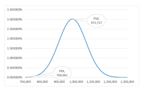
A couple times people have asked me to make a graph of the probability distribution. I struggled with this and in the attached file you can see how I made the graph below. You need the standard deviation and the P50 or average. Later in this page I describe how to compute the standard deviation using the mean squared error and assuming that different sources of variability are completely uncorrelated. Given the mean and standard deviation, you can first compute a minimum and maximum with the NORMINV function and a very small and a very large probability. Then you can make a range of values between the minimum and maximum. Once you have the values, make and x-y graph using the values as the x-scale and use the NORMDIST function as the y-scale. When you use the NORMDIST function, make sure the values add to 1.0. You may have to normalise the values through dividing by the sum. You can change the distribution and get a new graph and add P90 and a lot more stuff.
.
.
General Discussion of the Performance of Wind Studies and Use of Wind Production Probabilities in Debt Sizing
The graph below taken from a Fitch report demonstrates banker fear and problems with measuring wind probabilities. The graph shows the P50 and P90 case as well as the actual wind production. It is one of my favourite graphs in renewable energy analysis (much better than the famous solar efficiency graphs or graphs of which country has the highest penetration of wind and solar). I also like that the lines are all the same colour so that you have to spend some time figuring them out. We can start with the P50 case. As the P50 was made before the Breeze 2 facility went into service, it is a smooth line. The highest line on the graph must be the P50 case. When computing P90, you should realise that the P90 will be below the P50. The P90 in a sense lowers the production level until you can be sure that you obtain a 90 percent change of being correct. It is like a downside case where you only have 10% chance of being even worse. The amazing part of the graph is the bumpy line which must be the actual case. This is below the P90 in just about every time period and during the high wind periods, it is way below the P90 (perhaps there was not enough transmission to move power from the wind farm to the load centre). The title of the graph should be something like “Beware of Wind Consultants” or “Consultants are full of Sh…” You can find the recent actual production in the database presented at the bottom of this page.

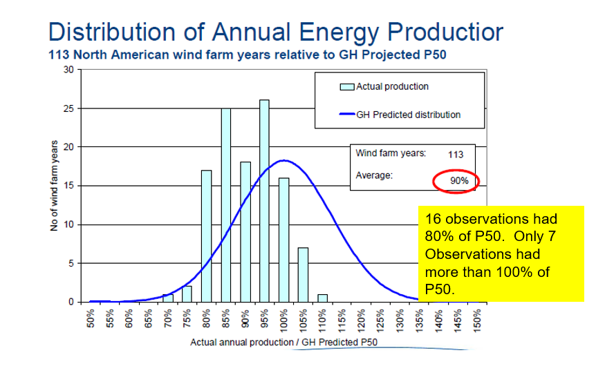
The next graph I present to introduce the subject is from Garaad Hassan, a very big consulting company. This graph compares the P50 estimates (shown for some reason as the blue line on the graph), compared to actual production. You can see for example, that for about 16% of the cases, the actual was only 80% of the projected — a decline of 20%. On the other hand there were only abut 6 or 7% of cases where the actual production was higher than the P50 case. The 80% case can be translated into the DSCR using the formula, required DSCR = 1/(1-Pct Change) or 1/(80%) = 1.25. (Test this out with DSCR-1/DSCR = .25/1.25 = 20%.
I have found recent estimates of for multiple wind farms where the P90 is compared to the P50. This shows a better result where the average production is similar to the P50 (although the P50 is still a little optimistic). The next screenshot illustrates the difference between P50 and P90 from real cases. The example shows that most projects exceeded the P90 level but generally, the P50 generation is less than the actual production. This demonstrates that P90 is reasonable for a downside case. But be warned that these projects are in similar locations with a good history of wind speeds.
This page explains how to evaluate the probability of achieving different levels of wind production that I refer to as P90, P99 etc. I also address the painful issue of the difference between a one-year P90 and a ten-year P90. At the end of the web page I describe how you can create financial models of tariffs and financing in the context of P50, P90, P99 etc. Measuring the probability of achieving electricity production from a wind project is central debt sizing of a wind project and the measurements are prepared before the financial close of a project. I demonstrate that the P90 or P99 often drive the level of debt. In describing P90, P99 etc. for the one-year case and the long-term case, I begin by reviewing some wind studies and describing two classes of uncertainty that drive the probability analysis. The first source of uncertainty is the variation in wind from year to year with the resulting energy production. The second is modelling error related to quantification of the production before the facility is operational. This second source of uncertainty related to modelling error is a lot more difficult to understand and define. With different sources of variation, I explain how to combine standard deviations (often called uncertainty) with one another using mean squared error. Once the mean squared error is defined the one-year and the ten-year (or twenty-year) P90 and P99 is established. At the bottom of this page I discuss incorporating the P90 and P50 in a financial model where the tariff may be derived from a target IRR on the P50 case and the financing could be derived from either a P50 or a P99 or a P90 case and the financing could further be derived from either debt to capital or from DSCR.
The tricky part of the P90, P99 etc. is to understand the sources of variation in wind production estimates that are mean reverting and that are related to modelling errors that do not self-correct. The first part of this webpage reviews general also describes general issues with performance of wind studies and debt terms related to probability levels of wind. The second section demonstrates some studies of 1-year and 10-year P50 and P90 wind studies and how to use the NORMINV function and the mean square error statistics. The discussion on this web page builds from the prior web page that dealt with variation in electricity production arising from variation in year to year wind speeds that are described on the prior webpage. The additional sources of variation that come from factors such as modelling error, turbulence, wake measurement error, correlation with reference data, availability, environmental issues and other factors are demonstrated. This page explains how to put sources of variation together and evaluate wind reports. Power point slides that explain these concepts are in the file available for download below (these slides are the same as the slides for the previous page). A similar discussion can be found for solar power in the associated link to this sentence. Below the power point file button, I have included two files with financial models that evaluate debt sizing from alternative wind probabilities and the maximum debt to capital. The second file available for download includes the parallel model concept to resolve circular references. Videos that describe these files are below the buttons.
[wonderplugin_video iframe=”https://www.youtube.com/watch?v=9dsgXkQzlas” videowidth=600 videoheight=400 keepaspectratio=1 videocss=”position:relative;display:block;background-color:#000;overflow:hidden;max-width:100%;margin:0 auto;” playbutton=”http://edbodmer.com/wp-content/plugins/wonderplugin-video-embed/engine/playvideo-64-64-0.png”]
[wonderplugin_video iframe=”https://www.youtube.com/watch?v=z960VpNuxMw” videowidth=600 videoheight=400 keepaspectratio=1 videocss=”position:relative;display:block;background-color:#000;overflow:hidden;max-width:100%;margin:0 auto;” playbutton=”http://edbodmer.com/wp-content/plugins/wonderplugin-video-embed/engine/playvideo-64-64-0.png”]
[wonderplugin_video iframe=”https://www.youtube.com/watch?v=762anHYXYPE” videowidth=600 videoheight=400 keepaspectratio=1 videocss=”position:relative;display:block;background-color:#000;overflow:hidden;max-width:100%;margin:0 auto;” playbutton=”http://edbodmer.com/wp-content/plugins/wonderplugin-video-embed/engine/playvideo-64-64-0.png”]
General Discussion of the Performance of Wind Studies and Use of Wind Production Probabilities in Debt Sizing
The graph below taken from a Fitch report demonstrates banker fear and problems with measuring wind probabilities. The graph shows the P50 and P90 case as well as the actual wind production. It is one of my favourite graphs in renewable energy analysis (much better than the famous solar efficiency graphs or graphs of which country has the highest penetration of wind and solar). I also like that the lines are all the same colour so that you have to spend some time figuring them out. We can start with the P50 case. As the P50 was made before the Breeze 2 facility went into service, it is a smooth line. The highest line on the graph must be the P50 case. When computing P90, you should realise that the P90 will be below the P50. The P90 in a sense lowers the production level until you can be sure that you obtain a 90 percent change of being correct. It is like a downside case where you only have 10% chance of being even worse. The amazing part of the graph is the bumpy line which must be the actual case. This is below the P90 in just about every time period and during the high wind periods, it is way below the P90 (perhaps there was not enough transmission to move power from the wind farm to the load centre). The title of the graph should be something like “Beware of Wind Consultants” or “Consultants are full of Sh…” You can find the recent actual production in the database presented at the bottom of this page.
The next graph I present to introduce the subject is from Garaad Hassan, a very big consulting company. This graph compares the P50 estimates (shown for some reason as the blue line on the graph), compared to actual production. You can see for example, that for about 16% of the cases, the actual was only 80% of the projected — a decline of 20%. On the other hand there were only abut 6 or 7% of cases where the actual production was higher than the P50 case. The 80% case can be translated into the DSCR using the formula, required DSCR = 1/(1-Pct Change) or 1/(80%) = 1.25. (Test this out with DSCR-1/DSCR = .25/1.25 = 20%.
I have found recent estimates of for multiple wind farms where the P90 is compared to the P50. This shows a better result where the average production is similar to the P50 (although the P50 is still a little optimistic). The next screenshot illustrates the difference between P50 and P90 from real cases. The example shows that most projects exceeded the P90 level but generally, the P50 generation is less than the actual production. This demonstrates that P90 is reasonable for a downside case. But be warned that these projects are in similar locations with a good history of wind speeds.


How Wind Probability Estimates Affect Debt in Term Sheets
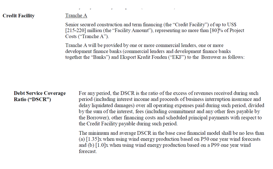
To illustrate how P99 or P95 or P90 can affect the size of debt I have included selected examples of terms from actual term sheets. The first screenshot is from a term sheet that was used for negotiation (i.e., before terms were finalised). The second screenshot was from a survey of how different banks would fund a project bid. At the bottom of the first excerpt, you can see that the debt size could be constrained by the P99 case where the DSCR for a one-year P99 case is 1.0. In the P50 case, the DSCR constraint is 1.35 (the term sheet erroneously refers to a 1-year P50 case. For the P50 average case, the standard deviation and probabilities do not affect the average and implies that the 10-year P50 and the one-year P50 are the same).
The DSCR of 1.35 in the term sheet example implies that as long as the percent difference between P99-one year and P50 cash flow is less than 25.92% (DSCR-1)/DSCR, the P99 case will drive the debt sizing from the the DSCR. (I put a few equations for this below the paragraph.) The second screenshot below the term sheet excerpt is from various different lender bids. This confirms that lenders have similar general terms with respect to DSCR’s on the P50 and one-year P99 in case you do not believe me. The equations I have put below the debt terms demonstrate how you could think about whether the P50 with a 1.35 constraint of a P99 with a 1.0 constraint would be in place. The last equation shows that if the P99 divided by the P50 production is less than 1/1.35 or .7408 (also 1-25.92%), then the P99 DSCR will be the driver of the debt size. This is why as a financial analyst or a financial modeller, you should understand wind probability cases. Here are some equations that illustrate how you can evaluate whether the P99 or the P50 will drive the debt size.
- Cash Flow P50 = P50 Production x Margin/MWH – Fixed Cost
- DSCR P50 (1.35) = P50 Cash Flow/Debt Service
- Cash Flow P99 = Cash Flow P50 * (P99/P50 Ratio) — If all costs are variable
- DSCR P99 (1.0) = P50 Cash Flow * (P99/P50 Ratio)/Debt Service
- If the debt size is the same in P50 and P99 –> DSCR P99/DSCR P50 = (P99/P50 Ratio)
Implication: 1/P 50 DSCR should be compared to P99/P50 if the P99 DSCR is 1.0
.

Introduction to one-year probability case versus ten-year or twenty-year case
In my opinion, the use of one-year P99 in the term sheet rather than 10-year P99 just means bankers look around for the worst possible number in the wind study; one-year production is less than ten-year production in cases such as P75, P90, P95 and P99. Please, please understand that the term 1-year P99 versus 10-year P99 does not have anything to do with how many historic years were used in estimating the probabilities. Nothing at all. What it does mean is that the 1-year probability includes two things. The first part is potential wind variation that can occur in one year. The second thing it includes is modelling errors that occur because the prediction is made before the facility starts operation and it may not work as anticipated. When you make a modelling error that does not reflect how the wind farm will really work (e.g. wake effects, turbulence effects, transmission constraints, availability), the error does not self-correct after one weather season. When there is variation in wind, this is mean reverting and not as much to worry about. A 10-year or 20-year P99 means that instead of worrying about fluctuations every year, you average out the wind variation that will move up and down and instead you average out the wind for 10 or 20 years. All of this means that the one-year P99 has two effects: (1) cyclical effects and, (2) permanent modelling errors. The 20-year P99 has one effect: the permanent modelling error.
Selected Examples of Wind Production Probability Estimates from Wind Studies
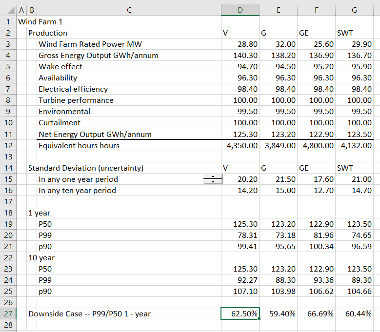
I have included selected examples of wind studies below in terms of the percent difference between the one-year P99 and the P50 case below so you can get an idea of whether the P99 or the P50 drives debt sizing from the DSCR. The first case presents a case where there was no good reference site and the difference between the P50 case and the one-year p99 case is large. When computing the P99 or the P90 in the above table, you can use the NORMINV function. The inverse part of the function implies that you begin with the probability and derive the X value which is just like the P99 value. You need the mean and the standard deviation along with the probability. This is a key point — when examining the probabilities, it all comes from the standard deviation. With the standard deviation defined in line 15 and line 16 in the screenshot below you can compute the lower values for the P99 and P90. For example, to compute the 1-year P99 of 78.31 in the first column of the screenshot, you can enter the function as follows using the P50 case for the mean and using the given standard deviation:
78.31 = NORMINV(.01, 125.3, 20.20)
Analysis of Multiple Wind Farms and Evaluation of One-year and Ten-year P90
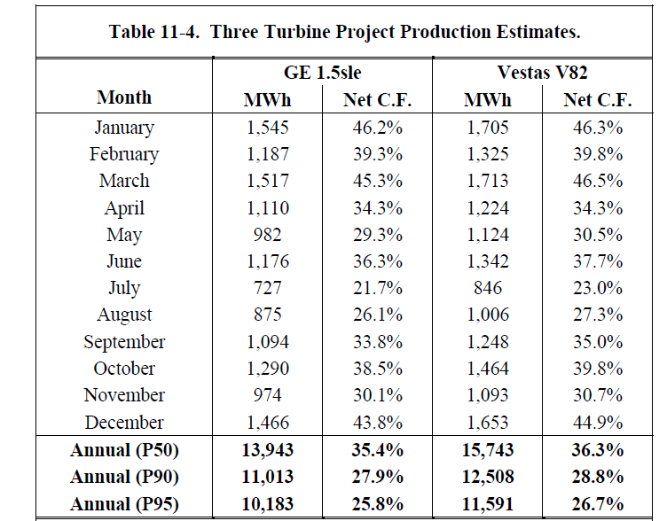
The screenshot below shows data from the credit report for different wind farms as well as the P95 and other cases after the read pdf process has been used. The screenshot shows the one-year P95 etc. as well as the 10-year P95 etc. for the different wind farms. Note first that the P50 case is the same for the 1-year case and the 10-year case. For the other cases, there is a bigger variation in the 1-year case than the 10-year case. You can see that P50 case is the same in all of the tables as the mean does not change. For example, in the case of the first farm, LB II, the one-year P95 is 270 while the 10-year case is 300, which is closer to the P50 case of 333. The 10-year probability case does not include cyclical changes and only includes uncertainty related to modelling error. When there a reduction in energy production because of modelling error, this error continues and does not have any reversion to the P50 case. The one-year case includes this permanent modelling error as well as cyclical differences that can make one year have a lower value because of cyclical wind patterns.
The percent difference between the P50 and one-year P95 is shown in the table. Note that percent difference varies between 82% for SW Mesa and 56% for the Montfort project. This implies that the required DSCR for SW Mesa to cover 1-year P95 wind variation would be 1/.82 or 1.22 for SW Mesa. The DSCR to cover the 1-year P95 risk would be 1/.56 or 1.79. The ratio of the 10-year to 1-year variation shows how much of the variation comes from temporary or cyclical wind speed changes versus how much comes from permanent modelling errors. If the percent 1-year to 10-year is 100%, then all of the error comes from modelling permanent error and none comes from cyclical effects. If the percent is lower, then the cyclical effects are relatively greater.
.

Deriving Standard Deviation from the Probability Estimates Using Goal Seek
The screenshot below uses the table above can be used to derive the P99 probability case. To do this, the standard deviation must be derived. You can derive the production for a P95 or P90 or P75 case with the NORMINV function in excel (in french LOI.NORMALE.INVERSE and in german, NORMINV, and in Spanish DISTR.NORM.INV). To compute production from the NORMINV function, you need the probability (which is given), the mean (which is the P50 case) and the standard deviation. The standard deviation is not known, but as I said above, it drives all of the probability analysis. You start by putting in some arbitrary number for the standard deviation. Then you can compare the computed production using the NORMINV function with the given production in the table. With the difference between the computed production and the given production for P95, P90 and P75, you can use the goal seek tool to derive the implied standard deviation.
Once the standard deviation is computed with the goal seek the P99 can be evaluated. Note that for all of the wind farms except the last Monfort plant, the standard deviation is the same whether the goal seek is made of P95, P90, or P75. This should be the case as the standard deviation is a given number. For the Monfort case, the change in standard deviation does not make sense and suggests there is something wrong with the data (note the change from 15 to 11 to 7 in column J and lines 13-15). The manner in which the goal seek can work across multiple rows and columns is demonstrated in the insert below.
.

Sub Mult_goal_seek()
'
' 1. Works for cells rather than range name
' 2. Can make loop with zero
' 3. replace row and col
'
For i = 0 To 3

   row1 = i + 23
   row2 = i + 13

   For k = 0 To 6
      col = k + 4

      Cells(row1, col).GoalSeek Goal:=0, ChangingCell:=Cells(row2, col)
    Next k
Next i

End Sub
Mean Reversion in One-year Probability versus Only Permanent Factors in Ten-year or Twenty-year Case
The key concept to understand is that the uncertainty that comes from modelling is not “mean revering” while the variation that comes from weather variation is mean reverting. The videos and files below address this subject that I find one of the most difficult issues to explain — i.e. the difference between one year P90 and ten-year or twenty-year P90. I have tried to explain this with file named “Wind Study” listed below. This file uses a nice old financial analysis report that listed P50, P75, P90 and P95 for a series of different wind farms. It also reported the production statistics on an 1-year basis and on a 10-year basis. Using the P90 etc. production statistics you can back out the standard deviation that is related to wind variation only as well as the variation that is only related to permanent effects. I have also compiled an analysis of the variability in wind after projects are operating relative to before they are operating. My key theme is that standard deviations underlying the ten year P90 are subjective. I demonstrate how to use the NORMINV function in excel to understand data in wind studies.
Understanding P90, P99 etc. in Wind Studies and Dissecting Wind Variation in Analysis with Mean Squared Error

.
Study in which you can dissect the one-year and ten-year P90, P99 etc.
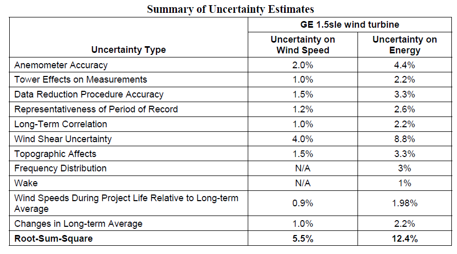
In the table above with P90, P95 etc. you need to have the standard deviation to compute the numbers yourself. If you want to compute P90, P95 etc. for one year versus 10-year you need to evaluate how much of the production of electricity from wind comes from the wind variation by itself. In this section I will demonstrate how this can be done and you can compute the standard deviation for the 1-year probabilities and the 10-year probabilities. Part of the reason for this is because you can have a better understanding of what causes variability and what causes the variation. After the variation is understood you can compare the wind only variation to the analysis discussed in the prior page. The first screenshot includes a row at the bottom named Combined Uncertainty. This is the mean squared error of the components above the row that include (1) anonometer accuracy, (2) wake effects, (3) correlation with the reference site and (4) wind variability. If you would simply sum the numbers above the combined correlation, you would not get the combined correlation. Instead, if you first square the numbers and then sum the squared numbers and then take the square root of the sum, you will have the number that is called the Combined Uncertainty which is the the mean squared error or Note that the mean squared error is described in the table. In addition there are separate components for the different items. To present data from this PDF file is a little tricky. It is a locked file and you can read it into google drive. Once it is in google drive you can use the read pdf file. The excel files associated with the tables are included.
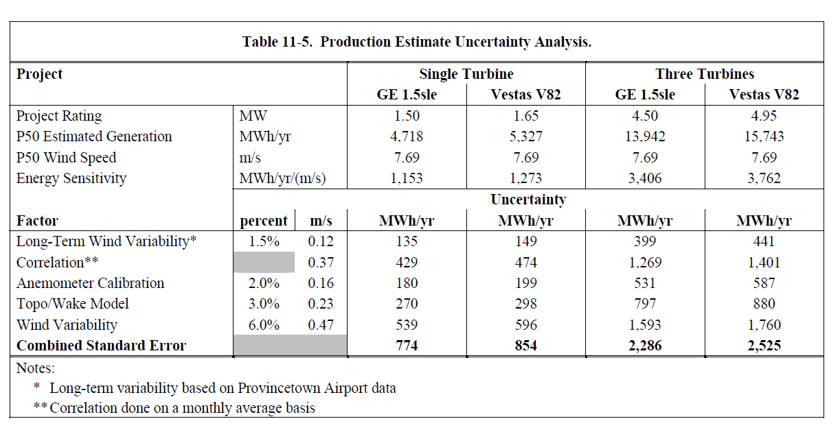
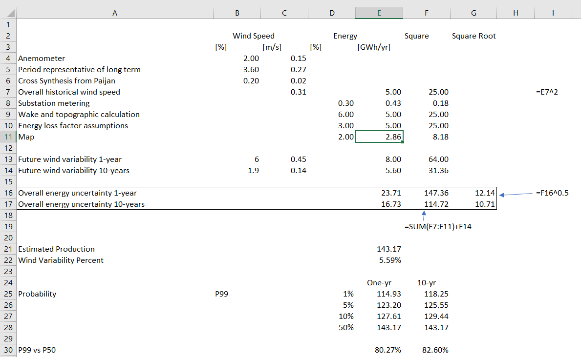
I have put an analysis of wind uncertainty that is presented in one of the wind studies into an excel file so that you can see how things are computed. You can download the second wind study by clicking on the button below. In the two screenshots below I have illustrated the calculation of 1-year and 10-year probabilities and shown a couple of formulas on the side. If you are really mean, you can question the consultants exactly where the uncertainty estimates come from.

.
MSE Simulation.xlsm
The general idea is that standard deviations underlying the ten year P90 are very subjective where standard deviation in things like wake effect, availability, turbulence, correlation to historic site, wind shear, losses and other factors. One of the main tools in analysis of wind production with different probabilities is use the NORMINV function in excel to understand data in wind studies.
Debt Sizing with Wind Probability Estimates (P99, P90 etc.)
As explained above, it has become standard in financing renewable energy projects to apply different debt service coverage ratios to different wind production cases. A typical scenario is that a 1.35x coverage ratio is applied to the P50 case while either a 1.2x coverage is applied to a P90 ten-year case or a 1.0x coverage is applied to the P99 one year case. The modelling issues can be a little difficult as the debt may be sized on one scenario but the equity IRR is computed from a different scenario. The exercise below applies these concepts.
.
Debt Sizing in a Financial Model from Either P50 or P90 or Max Debt to Capital while Deriving Required Tariffs from the P50 Case with a Target IRR
In this section I work through an analysis in which you compute that bid price from a P50 case but you compute the debt size my be derived from the P50 or the P90 or the P99 minimum DSCR’s or the maximum debt to capital ratio. I will walk you through this analysis in simple cases without taxes or circular references and then take you a more complex case with multiple debt issues, taxes, a DSRA account and multiple constraints. As with other subjects, I have provided an exercise file where you can fill in some of the blanks and also a completed file where you can see how things work. If you work through the exercise, you will have to create a macro with a goal seek function that computes tariffs at P50, then evaluates tariffs with different DSCR’s for P99 and P50 and debt to capital. After you compute the financing, you have to go around and compute the tariff again and the process iterates. The file attached to the first button below is a simple case without taxes and without circular references and a single debt issue where you fill in the blanks that are coloured with yellow. The second button has the simple case completed and the third file contains the multiple debt issues with all of the complications. This third file uses the parallel model concept and is explained in a separate web page that is linked to this sentence.
.
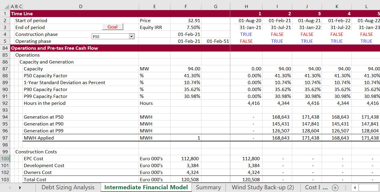
The structure of the simple file is shown in the screenshots below. I have created a simple model without a construction period or income tax (to avoid circular references) so that you can focus on the financial issues. The first file does not have any goal seek function to find the tariff or tariff setting from P50 and the debt sizing using alternative criteria. The wind speeds, capacity factor, probabilities and other technical characteristics come from an real wind study. Plant costs and O&M costs come from an actual financial model model. Basic inputs for the analysis are shown in the screenshot below. These inputs are combined with some financing assumptions that include the DSCR constraints and the debt to capital limits that were discussed above. The PPA price and the O&M expenses are assumed to increase with inflation. In terms of model timings, the construction period is assumed to be one year and the periods are assumed to be half year periods consistent with the interest and debt repayments. Debt repayments are assumed to be structured from sculpting. Once the inputs are established, the pre-tax cash flow is computed as usual by beginning with operations, moving to EPC cost and finally computing the pre-tax IRR. There are many examples of this on the website. For example, you can go to the A-Z project finance model and watch videos by clicking on the link associated with this sentence.
.
The first case is extremely simple. It does not work through any operating cash flow detail; it has a single debt issue and does not include a process which evaluates the tariff. The second case is still simple, but it includes some evaluation of wind production uncertainty; fixed and variable costs; computing P99, P90 etc.; debt fees; a grace period; and semi-annual cash flow. In this example you find the tariff from going to the P50 case, but you size the debt size in both the P50 case, the P99 case and from the maximum debt to capital. The third case includes circular references related to taxes, financing and the DSRA. This third file also includes multiple debt issues. It is one of the tricky issues in project finance, I think.
.
Wind Project Finance Model with P50 Case and P90 Case and Single Debt Issue with DSCR Theory
Very Simple Example of Debt Sizing Using Alternative Methods
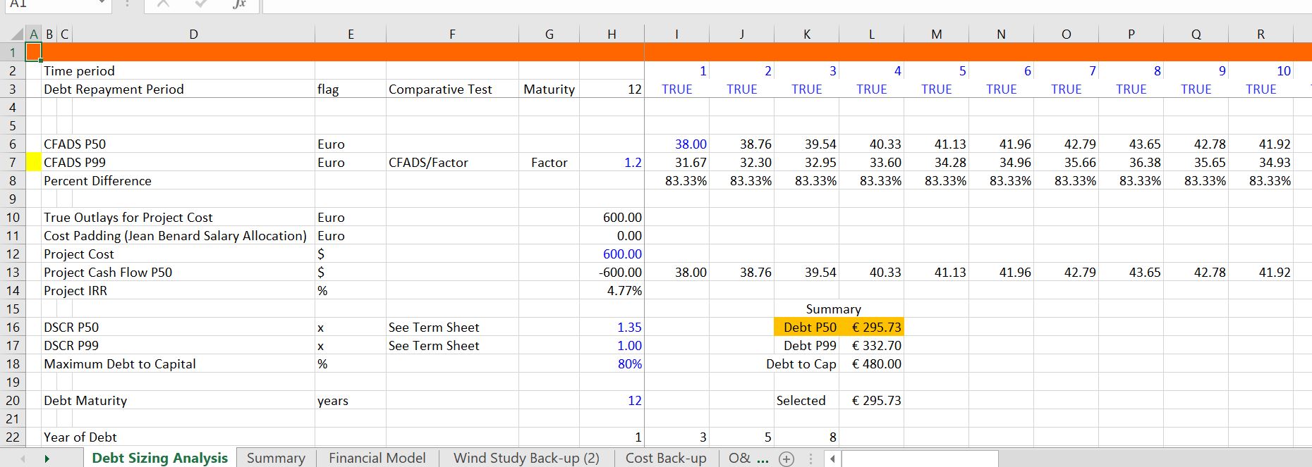
The first financial model example is very simple and I would like you to see a few examples that are progressively more complex. In the exercise file that are attached to the buttons below, you fill in the equations that have a fill colour of yellow. To size debt with sculpting, you need two formulas: (1) Debt Service = CFADS/DSCR and, (2) NPV of Debt Service is the debt at COD. These two equations for sculpting are essential in modelling and it is a big error to ignore the equations in creating a model. To compute the PV of debt service that is part of the second equation, you can use the SUMPRODUCT function. One of the small differences is that when you compute the compound interest factor, you should use the TRUE/FALSE switch to start the compounding at the first repayment date. Another idea that will be continued in other examples is that the debt schedule should be separate from debt sizing.
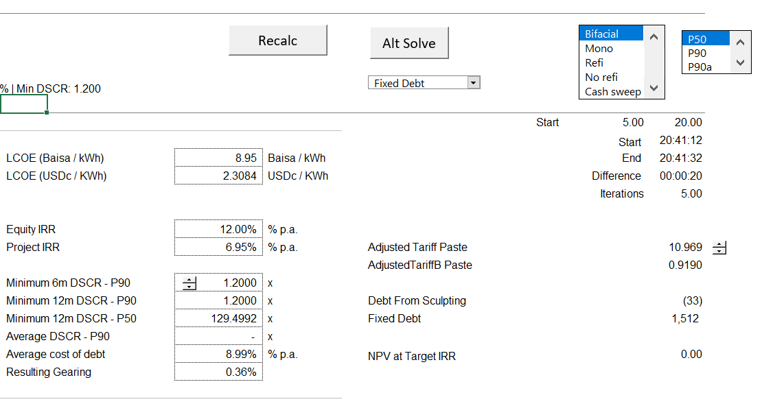
The simple debt sizing case that uses the two equations is illustrated in the screenshots below. In the excerpt there are two measurements of CFADS and the P99 CFADS is driven by the 1.2 factor showns in H7. Recall that if the ratio of P99 to P50 is less than the ratio of the DSCR in the P99 case divided by the DSCR in the P50 case, the P99 will drive the debt size. In this case the P99 divided by P59 is 83% while the ratio of the DSCR in the P99 divided by the P50 case is 1/1.35 or 74%. This means the P50 DSCR will drive the debt sizing. You could also compare the 1.35 difference in DSCR to the P50/P99 which is 1.2. If the DSCR ratio is greater than the CFADS ratio, the P50 will drive the debt sizing. In the screenshot below I also show the maximum debt to capital constraint. If the debt size from the debt to capital constraint is less than the debt that comes from the CFADS calculation will drive the analysis.
The next screenshot illustrates how you can compute the debt size from the alternative methods. Note that you should compute the debt size three times. The first is computing the debt size from the debt to capital ratio. This is just the total project cost multiplied by the maximum debt to capital ratio. The second method is computing the debt size from the NPV of the cash flow in the P50 case. The third case is computing the debt size from the NPV of cash flow in the P99 case. Please note that this case only works in my fake case that does not have any circular references. There is no construction period with IDC; there are no fees; there is no DSCR; and, there are no income taxes or interest income that cause circular references in the sculpting cases.
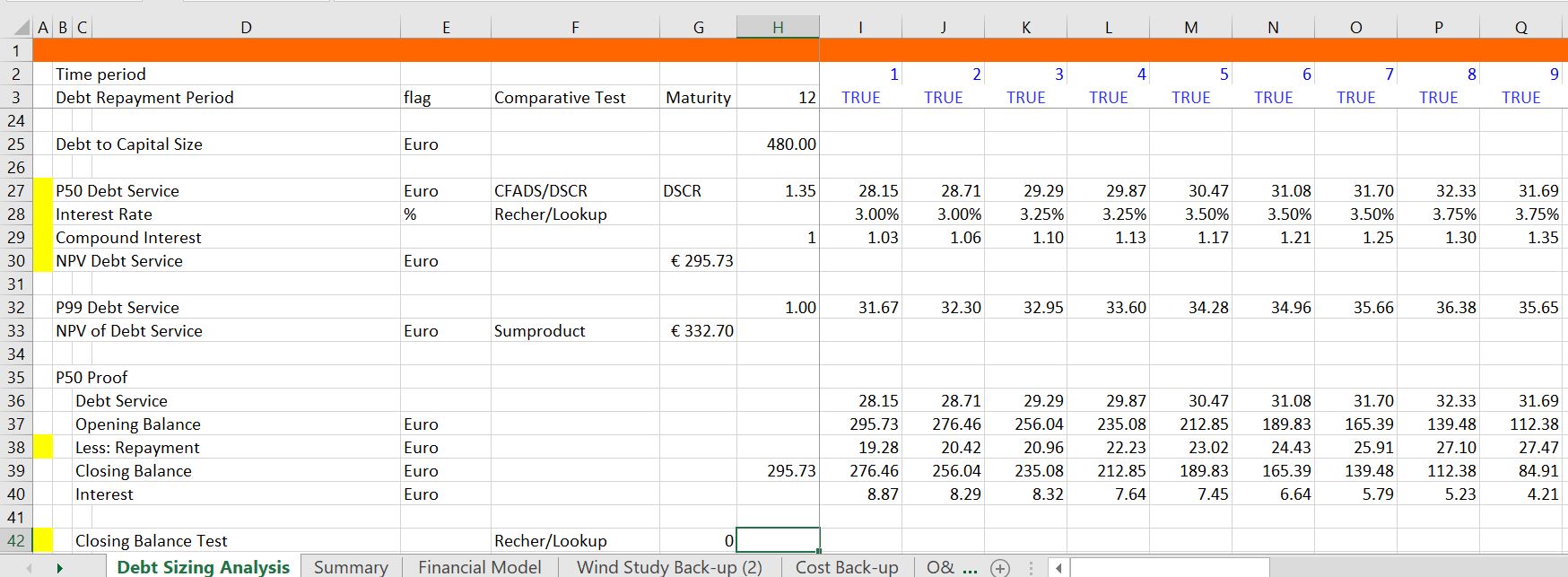
Once you know the NPV formula, you can compute the NPV of debt service with the different cash flows and the different DSCR’s. Then you compare the debt sizes from the different cash flows with the debt size from the debt to capital ratio. That’s enough for the simple case. Similar equations are in the more complex files with and without circular reference resolution. I will not make you go through the equations again but they are absolutely crucial.
Intermediate Case of Debt Sizing and Required Pricing
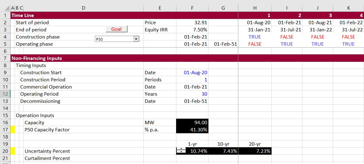
The prior simple case begins with CFADS that has an assumed P50 and P99. In the next file, you evaluate the derivation of P50 and P99 from a wind study. You change some of the key factors that derive the standard deviation that is the basis for probability estimates. Then, after evaluating the P50 and P99 etc., you use the goal seek to compute the required price with different debt sizes and different standard deviation estimates. Some of the ideas in this model are to understand how the P99 and P50 works with NORMINV from the standard deviation; to see how the fixed and variable cost affect the P99 and P50 analysis with different DSCR ratios; and to evaluate required tariffs under alternative uncertainty and standard deviation assumptions. The items that are discussed in detail and that you can work with in the exercise file are the items with the little yellow marker. In the first screenshot that introduces the model, you should enter the p50 capacity factor from the wind study. You can see how the one-year standard deviations are higher than the standard deviation estimates for the 10-year case and the 20 year case.
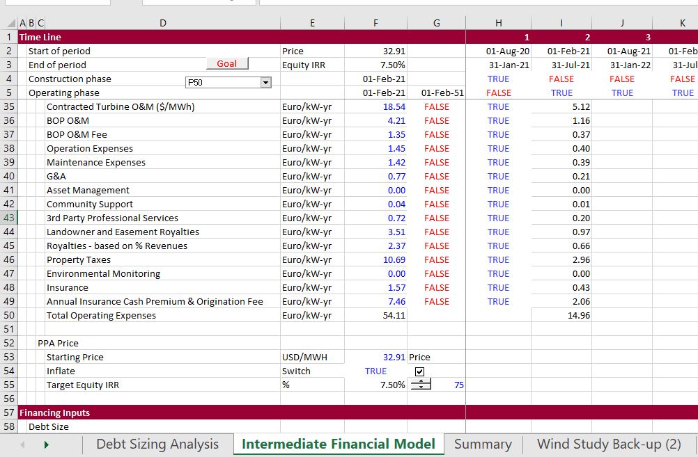
The second screenshot illustrates operating expense with TRUE and FALSE switches. The idea of this is to illustrate the effect of variable versus fixed costs on P50 and P90 and P99 etc. If the production quantity changes and all costs are variable, then the decline in variable costs off-sets the cash flow effects of the decline in volumes. But if the costs are fixed, the decline in volumes (and therefore revenues) has a bigger effect on cash flow. To evaluate this, You can change the costs either fixed or variable by changing the FALSE in column G.
The next screenshot shows that you should compute each line that can drive the debt size. In this case, the debt size can be driven by P50, P99 or P90 depending on the relative level of production and the difference in the DSCR used to size the debt.
The next screenshot works through sizing debt from the various production estimates. The production estimates are translated to cash flow by multiplying the production with the margin per MWH.
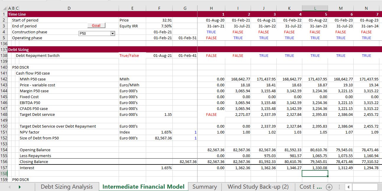
The next screenshot illustrates how to compute the repayment once the debt size is established The model currently uses the LLCR method where the LLCR = PV of CFADS/Debt Size Determined. The debt size is the minimum of the P99 DSCR, the P90 DSCR, the P50 DSCR and the maximum debt to capital ratio. The LLCR is then used to sculpt the debt.

The final screenshot illustrates the equity cash flow that is used to use the goal seek tool.

Advanced Case with Resolution of Circular References
In the more complex case, I have included taxes, monthly construction, DSRA accounts, interest and fees during construction, development fees, re-financing, equity bridge loans, and even an interpolate function. Once you have done the hard work of verifying your model with the parallel model, you can use the goal seek function to evaluate the tariff with the P90 and P50 problem. To see how this works I will walk you through the model and how to attach not one, but two parallel models. One that is attached to the P50 case and another that is attached to the P99 case.

Case with one debt issue and
P90, P99 and DSCR Debt Sizing.xlsm
P90, P99 and DSCR Constraint.xlsm
Wind Uncertainty Analysis from Analysis of Actual Plants
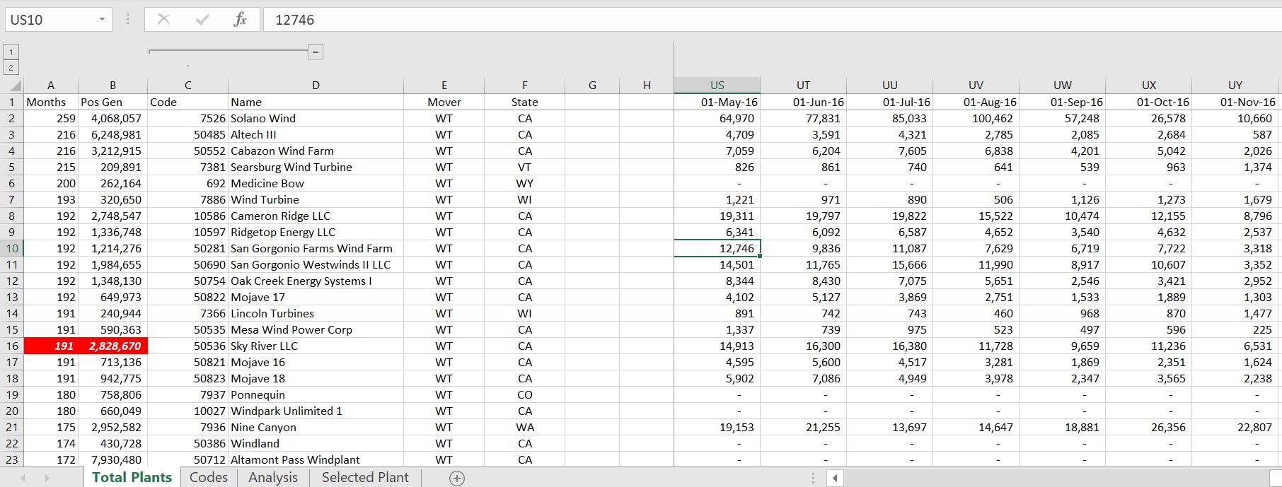
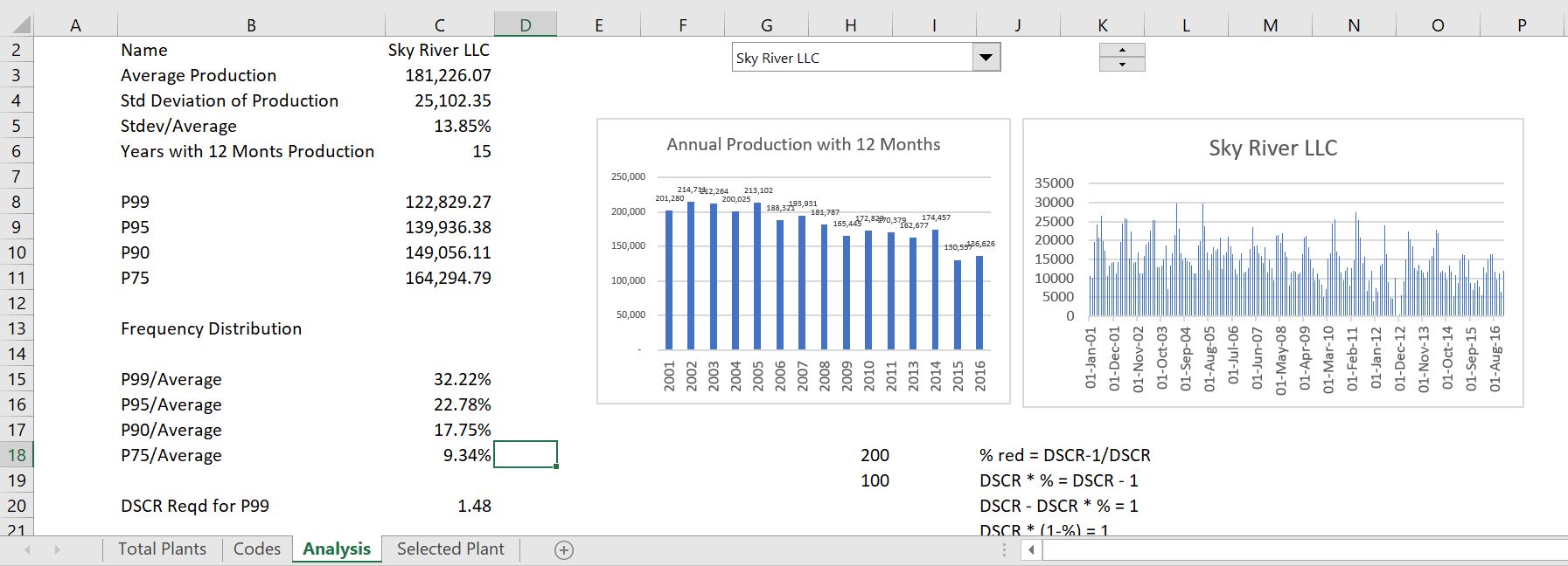
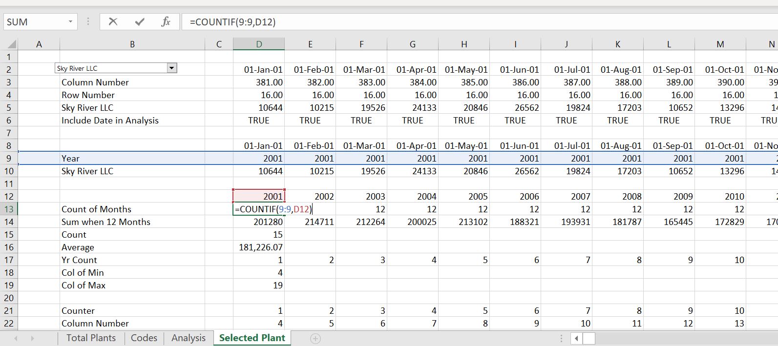
I have created a database of actual wind projects that contains actual historic production data on operating wind projects in MWH. In the U.S. the Energy Information Agency collects data on every power plant production by month (some plants do not seem to report in some years). I have used the month by month data and converted the data to annual uncertainty in order to evaluate the actual year to year uncertainty. There are some natural problems with this analysis. First, the configuration of the project may change. Second, there are not a lot of projects with long-term data. I am in the process of adding capacity to the database so that you can evaluate the capacity as well as the production data so you can see the capacity factor. I have put a similar file in the solar analysis section and the hydro analysis section. The hydro section has much more data. You can download the file by pressing the button below. I have put a couple of screenshots below the button to download the file. The screenshots illustrate the data collected from the EIA and the analysis made with the data.
.