This sheet explains how to construct a project finance model or a corporate model for a mini-grid or a micro grid. A mini-grid or micro-grid can be a village in Africa, a hotel in Berlin or anywhere that a grid is self sufficient and has no connections to a large grid. A mini-grid will generally have a portfolio of different generating assets, distribution assets and may have storage facilities. Modelling a mini-grid can seem to be very complex especially when you get a large project finance model. When modelling a mini-grid you are not modelling a single project. You are instead modelling an entity that has both demand and supply. Mini-grid modelling can seem to be quite complex where you have to add up demands of households, estimate energy generation, compute the costs of alternatives, make a project finance model, account for distribution costs, incrorporate battery storage and other items. In fact modelling, a mini-grid is like a mini-utility company — a mini Meralco, Tenaga, EDF or ConEd.
As with other files and analysis, I regularly update the files as I learn more from students and others about various details and procedures. In the case of mini-grids I have now seen more models (some of my collection is available on the google drive that you can get by sending me an email to edwardbodmer@gmail.com). I try and put the more recent files at the top of the page like the one below that includes detailed hourly data, load growth, solar details, components of battery analysis, load shapes, replacement scenarios and other things that you should have if you want to make a reasonable analysis of a mini-grid. I argue that the mini-grid analysis is really a corporate analysis and you must get away from the burecuratic crap of always only thinking about project finance models. This model has a lot of standard modelling techniques and can be applied to a lot of other analyses. Powerpoint slides that describe how the model works and the model itself is attached to the buttons below.
.
.
.
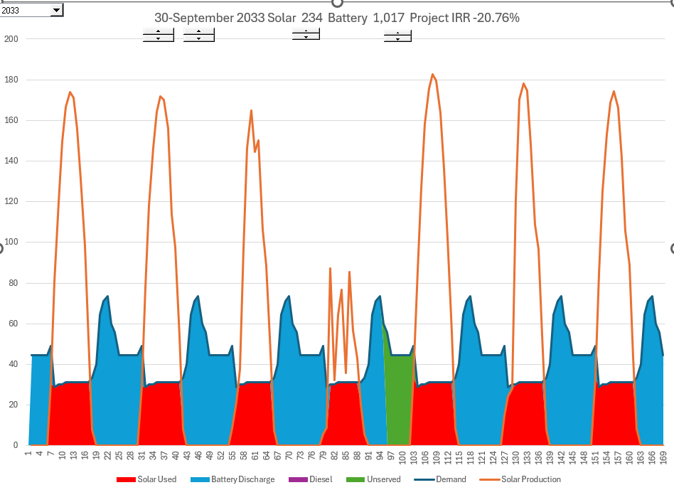
A couple of graphs from the hourly analysis portions of the model are shown in the screenshot below. I go crazy when somebody tells me that mini-grid modelling is simple. Modelling of a mini-grid allows you to think about the future of electricity systems without fossil fuel which is a variable cost. The graphs show the situation where there is insufficent demand to discharge the battery. The model allows you to select different mini-grids and apply different load shape, load growth, solar resource, battery characteristics and other operating parameters. These are combined with cost estimates to derive financial analysis.
.
.
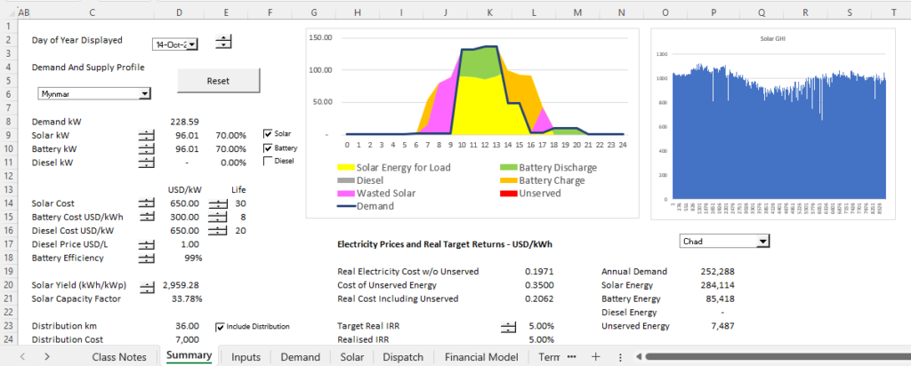
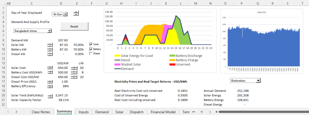
The solar resource is shown in the graph below. It is derived from PVGIS and can be benchmarked to actual solar data.

.
The solar is combined with loads and storage to derive the amount of load that can be met with batteries and the amount of load that is not met from renewable energy.
.
I suggest that when modelling an integrated utility company you would use a corporate model and not a project finance model. It is a corporate model because of continuing capital expenditures, replacement capital expenditures, financing and other items. You would have to understand the demand and energy balance, you would determine revenue requirements from the regulated cost of capital and there would be continuing capital expenditures. This is not how a mini-grid model is typically modelled. I use this model to illustrate how to be creative in making a presentation of how models work. The pictures below illustrate different demand profiles and different battery characteristics. Two models are attached to the buttons below:
.
.
.
.
Mini-Grid Model with Mini-Hydro and Diesel and Battery and Solar with Detailed Demand Build-up
.
The elemets of creating a mini-grid include:
- Setting up inputs derived from the number of households
- Include hourly demand profiles
- Include costs of different capacity options and amounts of capacity
- Include distribution costs
- Creating an hourly solar generation analysis
- Modelling hour by hours dispatch from demand profiles and solar analysis
- Start with demand
- Solar is next and find surplus solar
- Set-up battery balance with minimum constraints
- Model remaining load and diesel or other thermal
- Create Financial Model
- Start with Number of Customers and Demand
- Move to Load and Capacity Analysis
- Then you put in the capital expenditures
- Include retirements
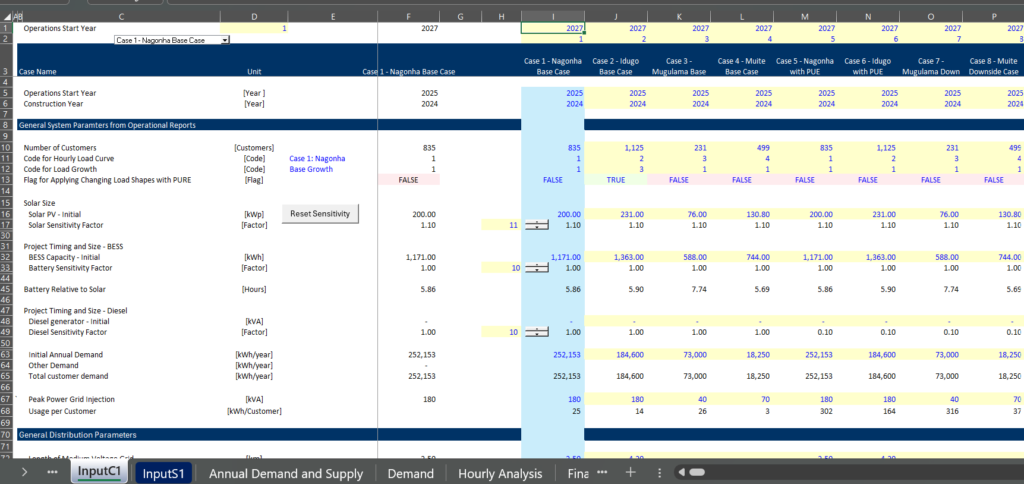
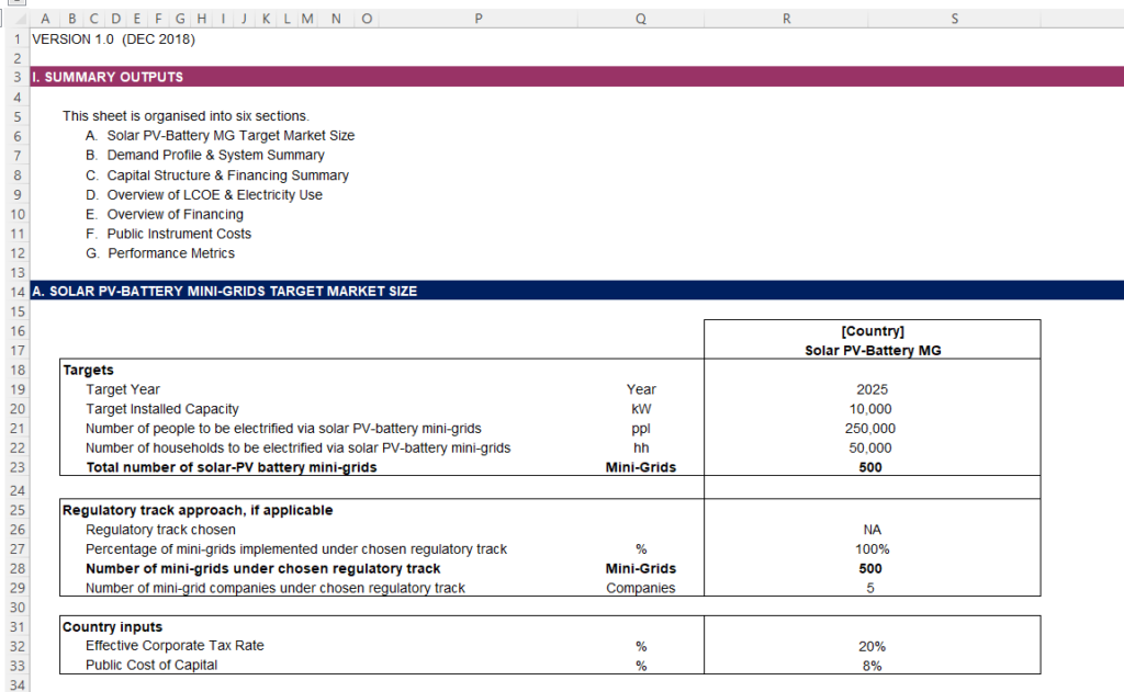
I suggest that you get a summary page that tells you what is going on while you are working on the model. This should allow you to evaluate whether things make sense when you are working on the model.
Start with Supply and demand inputs as illustrated below.

.

.
.

.
Demand
In the other file I worked a lot on the demad by adding together the lightbulbs and the fans and other things at each household. The assumption is that households will not change their behaviour when resources are avaiable (for example, charging batteries when the sun is shining). This can take (and waste) a lot of time. So for this exercise, I just take some hourly demand estimates from other sources. When you do this, you could also add some uncertainty with Monte Carlo simulation.
An example of estimated demand is illustrated in the screenshots below.
Start with Solar Resource
When you will create the model, you will want to make an analysis of the solar power. With the hour-by-hour solar you can combine the demand and the solar power to evaluate how to meet (or not meet) the remaining demand. You need to get the solar resource and make adjustments for the performance ratio to evaluate this hour-by-hour solar power that you will combine with the demand. I have used the solar analysis on an hour by hour basis from the UN model. It is nice because you can go and get the hour by hour solar from the PV GIS website.
Combining LCOE Concepts in the Mini-Grid Model
Some models compute the LCOE in the model separately and the put the LCOE’s in the model. My suggestion is to use LCOE concepts where the capital costs are based on the life, return and the cost in the model.
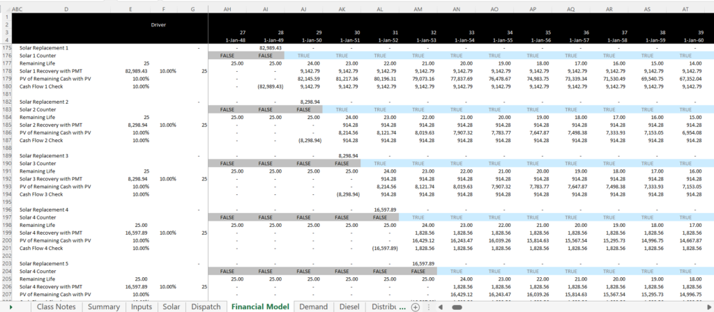
Computing Terminal Value
One of the painful things to do if you want to prove that your computations of PMT and economic depreciation are correct is to compute the terminal value. In this case you cannot compute the terminal value from some kind of model where you divide by the discount rate minus the growth or something similar. Instead, you can go through asset by asset and compute the remaining present value of the payment. Then you can add the present value of the remaining payment in the terminal period. The formulas include:
- Derive the replacement expenditures from the OFFSET function
- Replacement = OFFSET(Capital Expenditure, 0 , – Life)
- Put the replacement in separate line with AND relative to the prior replacement (the first formula is different)
- Note the vintage structure in the screenshot below
.
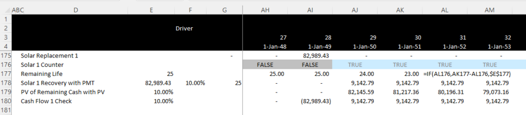
- Create a counter and the remaining life of the asset
- Use an AND function to with the prior flag and the first time you find a positive capital expenditure to create a counter
- This should be the period after the first capital expenditure
- The manner in which you compute the remaining life is shown in the screenshot below.
- Compute the PMT that will recover the total capital expenditures
- Use the PMT with the total capital expenditure (shown in column E)
- See a full explanation of the PMT formula in the LCOE section
- You can make this adjusted for inflation, degradation and taxes
- See more detail that the page https://edbodmer.com/real-lcoe/