An on-line project finance modelling course is presented through videos, excel files and screenshots on this webpage. This on-line project finance model course is structured to include both theory and practice where the project finance and/or modelling theory and/or accounting is discussed before working through technical modelling issues. The course covers advanced topics related to depreciation, development fees, debt structuring, circular references, multiple debt issues and sculpting and DSRA complications. The course is presented below with a series of videos and associated files as well as a set of power point slides. You can look at the completed files or you go to pages where you must enter various key formulas in the excel file to become comfortable with the analysis.
If you are starting out in project finance modelling and have not yet made a project finance model, the files and videos below are intended to allow you to see the project finance structure, the importance of timing mechanics, the essential nature of separating operating cash flows from financing cash flows and other issues including cash flow waterfalls. I have seen people try to learn modelling by copying various techniques from large actual models. This is a complete B.S. way to learn modelling. The models are often wrong, and worst of all, young people waste time on the format of the models without understanding key principles. The set of videos and associated files also introduce you to some important and difficult financing issues related to raising funds during construction, evaluating debt size using different approaches, simulating different repayment and re-financing and measuring the effect of credit spreads and interest rate hedging. As soon as you start modelling debt you will hit a wall because of all sorts of circular references that can mess up the analysis. Instead of using typical copy and paste macros after you hit the wall, the on-line course below uses an advanced user-defined function approach to resolve the circular references. Using the UDF is the key to advanced project finance structuring analysis.
.
Instructions for Downloading Files with Macros
.
Learning Project Finance Modelling and TLNV or TLNR
If you want to learn project finance modelling in half an hour you can build some sort of crude model of a solar project. This may be good enough for your interview or for a simple analysis of a project. But you will not have any deep understanding of the nuances that arise in both project finance theory and the associated project finance models. If you want to become a good modeller, you need patience and you cannot watch a few five minute videos from your phone on the metro (as you cannot learn from large actual models). Because of the complexities in modelling and in understanding the theory, the videos presented below are long. A lot of people tell me about Too Long Not Read (TLNR) or the perhaps the cousin Too Long Not Viewed. This is because I am taking you through a complete project fiance model.
After I published my exciting 634 page novel on project finance modelling, I made a lot of videos to go along with the subjects in the book. I did not make the videos in a very professional manner — too much dog barking in the videos, music in the background and too much swearing. Most importantly, the videos did were difficult to follow, they did not have any real theory as to why you are following various procedures and they did not have examples of what not to do. I received comments about background music, quality, lack of professionalism etc.. So now I have slowly started to make a set of revised videos. My friend Fredecrico from the Green Climate Fund told me it was Sh….
There are a few files that are necessary or helpful if you are brave enough to work through the lesson set. One file is a power point file that is referred to in the videos and that documents the modelling techniques. The second file is the excel exercise file that goes along with the on-line course where you can try and enter formulas for the blank rows. You can download theses files by clicking on the buttons below.
Power Point Slides that Accompany Project Finance Modelling A-Z Analysis and On-line Course
The first four parts of the course do not even include debt, but go through the financial modelling, timeline and structure of a model which are essential ideas.
Introduction to Course, Modelling Principles and Key Functions
The first part of the course just reviews some modelling principles of being lazy with excel formulas; looking at some bad practices in other models and discussing some theory. I also included a couple of files that you can use to prove if certain practices make a file “heavy.” A “heavy” file may be too big or it may be too slow. In the file that you can download by clicking on the button below, you can test whether an excel practice of clicking on an entire line slows excel down or makes your file larger. The answer is that using an entire row or column with LOOKUP and/or INDEX does not. Files associated with the video that prove the size and the time issues can be downloaded by pressing the buttons below.
Excel File that Tests Size and Speed of SUMIF Function with and Without Using Entire Lines Input
Excel File that Tests Size and Speed of LOOKUP Function with and Without Using Entire Lines Input
I am creating these exercises for a course I am teaching so that participants can review the subjects and the participants can test their knowledge. The very nice person who arranged the course also asked me to include some modelling behaviours in project finance that are disgusting. I have also discussed these practices in more detail on the A-Z page that is linked to this sentence. The only excel function to use in the first example is the LOOKUP function (VLOOKUP and HLOOKUP are illegal). En francais, cette function est RECHERCHER. I have included a sheet with bad practices so you can correct them.
High Crimes and Misdemeanors in Project Finance Models (All of Us Have Been Guilty)
All of the financial modelling companies seem to have their blah, blah, blah acronyms and rules. For what it is worth, here are some of my comments (not necessarily rules). I don’t tell you what to do; I tell you what not to do and the focus is making the models easier to understand and work with. I tell you this because I have made all of the mistakes and I have stole both bad and good ideas from many other models. After making mistakes, I believe these things really work. But one of my biggest complaints is paying too much attention to the rules and applying so-called best practice rules.

- Obviously, no hard-coded numbers after assumptions in the model. This is a clear crime and an even worse crime is mixing a formula with hard coded numbers like F5 * 1.02. The first can be solved with F5, paste special, constants or with Generic Macros.
- Not putting driving factors in the left column. Why in the hell do people put the sums in the left column instead of the factors that drive the equations. It would be much better to show the factors that are driving the model.
- Not making formulas the same across columns, another obvious one. You can make the formulas the same across the columns with TRUE/FALSE or 1/0 flags, or whatever you call them.
- Wasting time on meaningful or meaningless colours is one of the most irritating things I have to put u
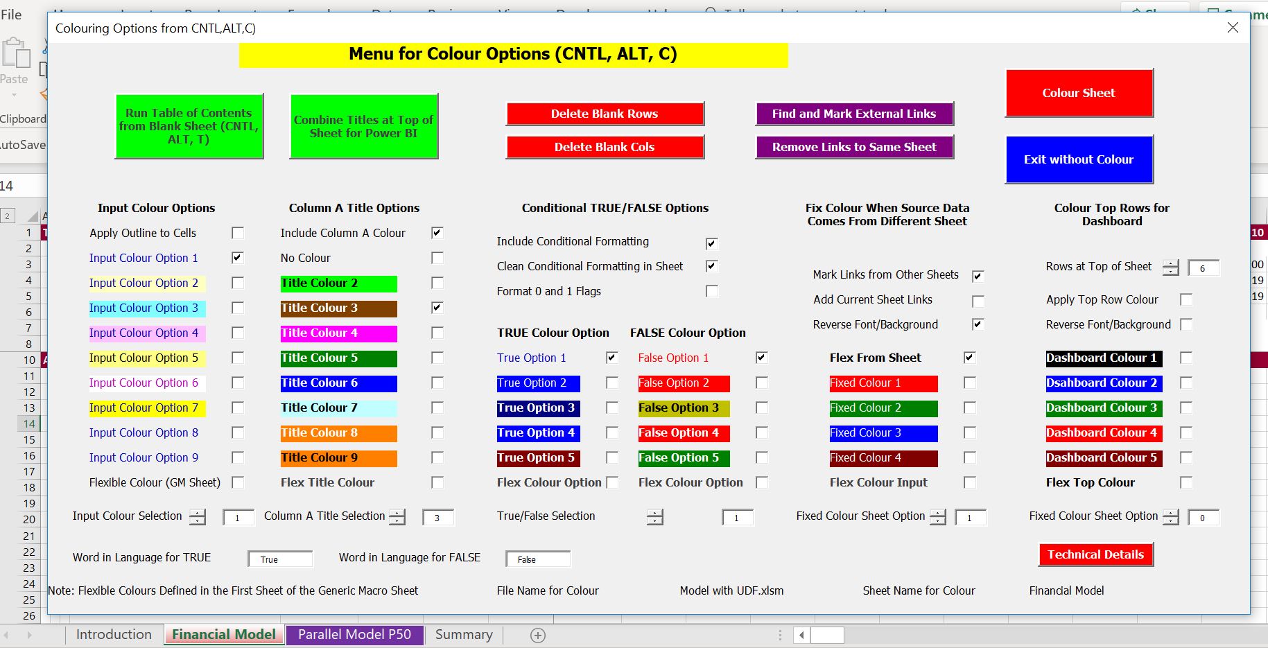 p with when I watch people make a model in excel. That is why I made the colouring page that allows you to find the location of other sheets and stop wasting time.
 - Use IF instead of MAX and MIN functions to connect the cash flow with the debt schedule. There is always a direct or indirect connection of the debt schedule with the balance sheet — no cash flow and no debt repayment. The MIN and MAX (never IF statements) should be in the cash flow waterfall and not in the debt schedule.
- Putting the Flags, Masks, Switches (whatever you want to call them) in a separate page instead of where they are used right next to the calculations. Why force people to make silly traces with those blue arrows to find things that are driving the model (even if they have a fancy add-in).

- Placing the forecast financial statements at the beginning of the model. Structuring is the biggest deal of FAST and other blah, blah, blah acronyms. You should the model with pre-tax cash flows, after-tax cash flows, summary sources and uses, debt sizing, debt schedules with repayment and interest and then, finally the profit and loss and the cash flow statement (the flow should be natural).
- Splitting up pages when you are designing the model instead of letting the model smoothly flow down a single page. I even think you should leave the model on a single page after you are finished and not split it up. Please put yourself in the position of somebody trying to understand the model. Your model should have a natural flow and it is so muc
 h easier to follow a model on a single page. Use little columns on the left so you can see the structure of the model.
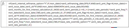
 - Deceiving yourself that you are smart because you make a long and complex formula. Use of formulas that are too long is inexcusable and always avoidable. The key to making models transparent is separating formulas and making them short.
- Showing off your excel prowess by applying unnecessary functions. You can do just about everything with three excel functions — LOOKUP, INDEX and SUMIF. LOOKUP is more efficient and easier to use than INDEX, MATCH and OFFS
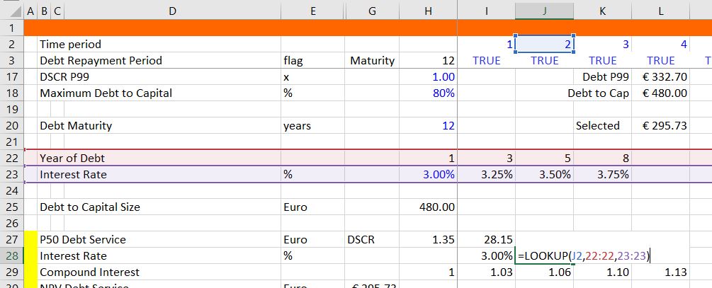 ET is unnecessary. When you use LOOKUP please click on the entire lines rather than wasting time fixing cells.
 - No formulas in the balance sheet. When you make a model all or the balances for debt, DSRA, net plant and other things should be in various structured sections of the model. The only balance that is not there in your model is the equity balance, which you should compute after the Formulas in the balance sheet rather than links to closing balance
- Don’t go overboard to show off your auditing skills. Use TRUE/FALSE switches for checking the balance sheet, debt balances and circular references, but you do not need to go overboard.
- Don’t pollute your fundamental models with multiple scenarios. Put the scenarios in a separate sheet (except P99 or P50) and let the scenario sheet be a mess with the index function and code numbers.
- Don’t make summary sheets complex. A simple rule is that output sheets can be deleted without affecting the model. This is pretty obvious that you do not want to mix outputs and inputs. Put
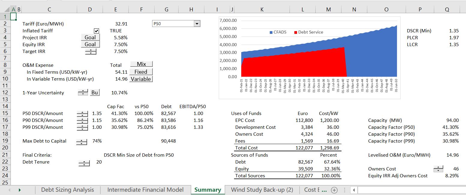 your summary on one page so you do not have to look around. Include IRR’s, DSCR, LLCR, a graph of cash flow versus debt service, a sources and uses summary and key drivers such as capacity factor, cost per kW, levelised O&M cost and the plant capacity. Then you can even call it a dashboard if you need to.
 - Don’t use the NPV or XNPV formula when interest rates are changing. Use a compound factor when interest rates are not constant and then compute the present value with the SUMPRODUCT function where you divide the cash flow by the compound factor.
- Putting forty flags at the top of a separate sheet sucks. You need an construction phase and operating phase at the top of your single sheet. But do not put too many of them at the top of a separate sheet (this will be very controversial for the dushbags who believe they are following some kind of best practice standards like SMART).
- Find a good style and don’t listen to me. I like the positive number convention. I like the using underlines for key items. I like using thin columns at the left.
- Take the side of Anti-Range Namers. The range name controversy is a subject at excel parties. There should not be an argument. Except for macros, range name suck. Some companies try to make you put range names in excel cell. This adds a log of time and if you have simple formulas, it adds nothing.
- Don’t chimp on sub-totals in the cash flow waterfall. Sub-totals are important in cash flow waterfalls. Connect the debt schedule with the sources and uses and also the cash flow waterfall. Why would you make people search for basic and obvious links.
- When using the goal seek tool, use the NPV = 0 rather than an IRR difference equals zero. When, the IRR cannot be computed, the goal seek can go crazy like we all know. As you know when the NPV is zero, the IRR is the discount rate. It is much better to use the NPV rule.
- Don’t compute the project IRR from CFADS. That is a basic mistake in finance theory; instead compute the project IRR before any finance equations are in the model.
- Work on the nightmare blue lines from circular references last. While working on your model, try to avoid circular references by doing things like using EBITDA instead of DSCR and construction expenditures instead of total funding uses.
Part 1: Timelines and Consolidating Periodic Periods into Annual or Quarterly Statements
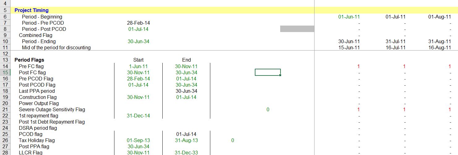
Developing dates and timelines and putting the timelines at the top of each sheet is a standard part of financial modelling and included in all of the regular old blah blah blah classes that you can get elsewhere. Formulas for establishing dates and switches (or flags or masks or whatever you want to call them) is very standard. One issue that is a bit tricky is being careful about annual analysis when moving from monthly to semi-annual cash flows.
For the fiscal year used in the annual page, you want to find the end of the month before the COD. You can just use EOMONTH function and enter -1 for the month — EOMONTH(COD,-1). Then find the month of this date using the MONTH function. Once you have the month end for the fiscal year, enter a switch that is true whenever the end month in the main time line is equal to that month. You should create the year of the date with the formula that the year changes when the fiscal month is reached. To do this use an IF formula — IF(MONTH(end date in time line) = Month End defined above, Year = year +1, prior year). This makes a year counter that increments whenever the fiscal year end is true. The process is shown in the two screenshots below. The first screen shot is really the key. Note that the commercial operation date is 1 August 2023. You need to find the prior month (including if the month happens to be December). This month can be used to drive the SUMIF function. Note that instead of using the function MONTH(COD) – 1 which would not work for January or December, you can use the EDATE with -1 for the month and then put the month around the EDATE. The formula is MONTH(EDATE(COD,-1)).
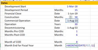
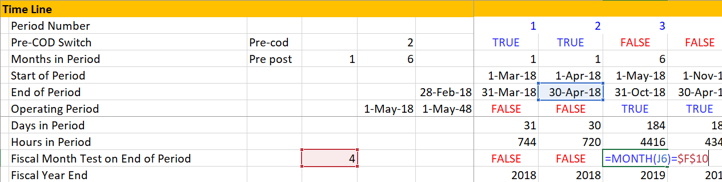
The second part of this method is shown in the screenshot below. In this example, the COD date using the standard monthly analysis is 1-May-2018. This means the fiscal year end will be April. But when the model switches to semi-annual mode, the month of April is in the ending date and not the beginning date. But you want the switch for a new year to start after the closing date. So you should take the PRIOR closing month and use that in the test. Once you have done all of this you can use the computed fiscal year end rather than the calendar year computed from the start or end date. The fiscal year is computed from the prior fiscal year and incrementing the year when the switch is TRUE.
Section 2: Volumes and Capacity and use of the Interpolate Function
In a model, whether an agriculture model, a model of a toilet paper factory in Jamica, a model of an airport or an electricity project, do not start with any thing that has money (Euro, USD, CFA etc.) Instead, start with the capacity and volumes and what the machine or the project is really doing. This is the subject of the second part of the course. In this section the INTERPOLATE UDF function is introduced to illustrate how to make volumes, capacity factor or other items gradually increase or decrease (a simple way to interpolate is not in excel). You can download a file with the interpolate function below so that you can add the function to any of your models and do interpolate really fast.
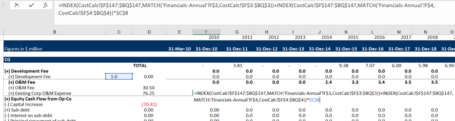
Problems with not using lookup or interpolate_lookup are illustrated in the screenshot below. In this case somebody thought they were really cool by using MATCH and INDEX together. But this just creates a long mess. It is much better to use the LOOKUP function with an entire line.
Section 3: Pre-Tax Operating Cash Flow
The third part of the course begins with some equations that involve money. In any project from a PPP for a University, a toll road, a co-generation plant or any electricity project, you should start with EBITDA and Capital Expenditures (and, maybe working capital). These items define the pre-tax project IRR of the project. With the pre-tax project IRR you have the essential information on the project. In this page I use the IRR even though I believe there are a number of problems with the IRR. To see a discussion of problems with the IRR you can go to my separate page that deals with the subject.
Section 4: Depreciation and Taxes to Compute Project IRR After Tax
The second set of videos complete the model with no debt and begin adding debt to the models. The last video in this section begins to add a circular resolution template to the model. This is an important idea in project finance where you would like to maintain flexibility in the face of natural circular references.
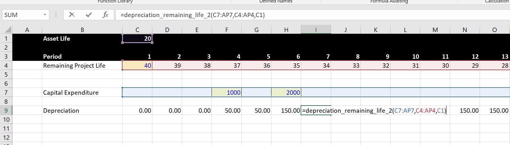
In adding on-going depreciation on future capital expenditures, I have included a function that enables you to select the entire line of future capital expenditures and remaining lives. With these data items and the lifetime of the equipment, you can derive the depreciation on future capital expenditures. The future depreciation is either from standard depreciation if the lifetime is greater than the remaining life. Alternatively it is computed from the remaining life when the remaining life is less than the asset life. A file that contains the function is available for download by pressing the button below (note that you have to press Shift, CNTL, Enter instead of enter and you cannot use the entire line). The file also contains a function that is more flexible and will simulate variable declining balance depreciation.
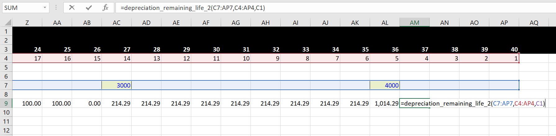
The screenshots below illustrate how to use the function with straight line depreciation. The first screen shot demonstrates how to function works in the case where the remaining life is greater than the asset life and the asset can be fully depreciated over the remaining life. In this case, the capital expenditure occurs in year 20 and the remaining life is 34 years. Note that two capital expenditures are entered and the depreciation stabalises at a level of 150. After the first asset is retired in period 24, the depreciation will fall to 100. The second screen shot shows the case where the remaining life is less than the asset life. In this case the depreciation is computed over the remaining life of the asset. The inputs for this function include the remaining life, the capital expenditure array and the asset life as shown in both screen shots.
The video below works through various depreciation and issues related to future capital expenditures and explains why the problem of future capital expenditures and depreciation would be very messy without a function. You would have to make one of those diagonal matrices and adjust for situations where the depreciation would expend beyond the life of the project.
.
.
The VBA code for the depreciation function is available for download below. Because this is a function, you must copy the code into your model rather than simply having the file with the VBA code open (with regular old macros you can do this). You can get this function with the VBA code into your project finance model in three different ways:
- The first way is to open the file above and press ALT, F8. Then edit the VBA page with the subroutine named A_Depreciation_functions. Copy the entire contents. After that, go to your sheet and press ALT, F8 again. Then create a blank VBA subroutine and copy the contents above that routine.
- The second way is to copy the function that is on the form that appears when you open the file. You just copy the code, go to your sheet, press ALT, F8, create a dummy macro and paste.
- The third method is similar to above, but you just copy the code from below.
Option Base 1

'''''''''''''''''''''''''''''''''''''''''''''''''''''''''''''''''''''''''''''''''''''''''''''''''''''''''''''''''''
'''''''''''''''''''''''''''''''''''''''''''''''''''''''''''''''''''''''''''''''''''''''''''''''''''''''''''''''''''
'''''''''''''''''''''''' Depreciation Functions
'''''''''''''''''''''''''''''''''''''''''''''''''''''''''''''''''''''''''''''''''''''''''''''''''''''''''''''''''''
'''''''''''''''''''''''''''''''''''''''''''''''''''''''''''''''''''''''''''''''''''''''''''''''''''''''''''''''''''

Sub A_Depreciation_Functions()

End Sub
Function depreciation_remaining_life_2(capital_expenditure, remaining_life, max_life) As Variant ' When the output is an array define as Variant

cap_exp_periods = capital_expenditure.Count ' See how many capital expenditure periods are modelled

Dim Depreciation_Expense(5000) As Single ' Make a new array variable that is the output
Dim remaining_life1(5000) As Single

' Determine whether to use remaining life or something shorter

For vintage = 1 To cap_exp_periods ' make a second loop to evaluate asset by asset
  If remaining_life(vintage) >= max_life Then
  remaining_life1(vintage) = max_life
Else
  remaining_life1(vintage) = remaining_life(vintage)
End If

Next vintage

For model_year = 1 To cap_exp_periods ' loop around each period and make a square with columns and rows

  For vintage = 1 To cap_exp_periods ' make a second loop to evaluate asset by asset

    age = model_year - vintage + 1 ' calculate the age of each expenditure (the diagonal)

    If (age > 0 And remaining_life1(vintage) <> 0 And remaining_life1(vintage) >= age) Then ' Only when asset is alive

      Depreciation_Expense(model_year) = _
      capital_expenditure(vintage) / remaining_life1(vintage) + Depreciation_Expense(model_year)
    End If

  Next vintage ' Note that the vintage is used for the capital expenditure

Next model_year

depreciation_remaining_life_2 = Depreciation_Expense

End Function

.
Section 5: Balance Sheet and Verification
The balance sheet is a good (but not perfect) way to check your model. A few years ago a student in my class told me that he puts a balance sheet into the model very early on in the process. At first I did not see the value in this. With complex models and solving circular references I think that suggestion was exactly on the mark. So much so that I put a test right at the top of the model and believe the saying on the t-shirt below from my friend Hedieh (you can order this t-shirt or a mug if you want. Just send an e-mail to edwardbodmer@gmail.com).

You can put the balance sheet into the model after you have modelled the depreciation expense. The balance sheet should just collect closing balances from other sections of the model. The video below describes the process of balancing the balance sheet before any debt had been put into the model.
This page includes an exercise where you build the financing part of a project finance model (i.e. starting with EBITDA) and then moves to the issue of resolving circular references. The first part of this page provides instructions on how to build the financing part of a model with flexible construction financing (pro-rata or equity first), sculpting of debt and a funded DSRA account. The exercise includes an associated video that explains how to work through debt sizing, repayment, interest and the DSRA from a file that includes blank titles. I use this exercise as a pre-course assignment in project courses that are advanced where I deal with nuanced issues of debt sizing, debt funding, debt repayment, debt cost of capital and debt protections. In these courses I don’t want to take time building an A-Z model and participants can assure themselves that they have the fundamental modelling skills. As this exercise includes circular references for IDC, DSRA and sculpting with taxes, a demonstration of how to implement the parallel model concept and resolve circular references is included. In order to focus on the tricky project finance issues, the exercise is for a case with a single debt issue in the context of an annual model. For the pre-course exercise, you should only focus on the first part of this page.
Section 6: Debt Financing in Project Finance Model – One Debt Issue with Simple Sculpting
I have made an exercise for adding debt financing to a model. The exercise begins with EBITDA and includes using a flexible method of up-front or pro-rata equity financing, computing IDC which causes a circular reference, creating repayments and debt sizing using sculpting with a given DSCR and programming equations for a DSRA account. I put the video explanation where I worked through the blank titles can created equations in the video below the button. If you are not using the video or the instructions below, please note that you should should use the horrible iteration button when it comes to items that cause circular references.
Part 1: Overview of Exercise, Colouring and Interpolate
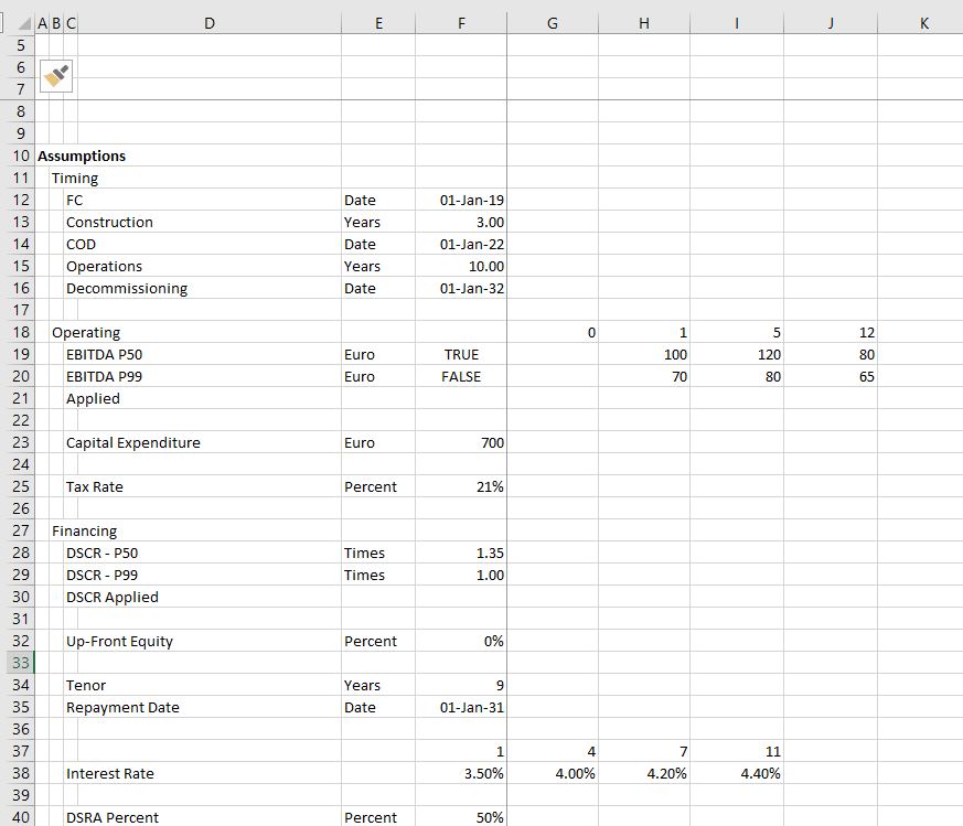
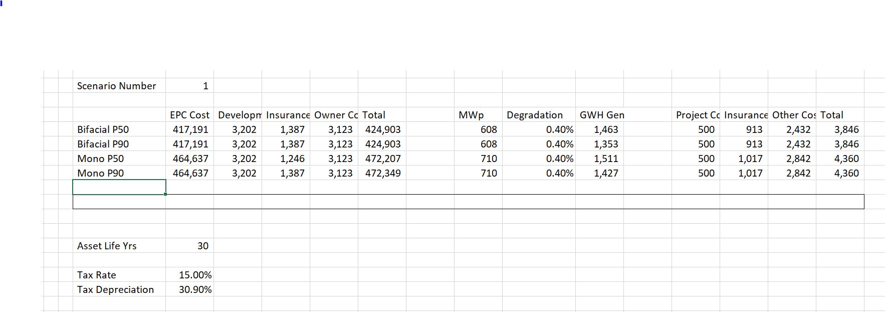
After you open the file, I suggest that you look over the inputs and the structure that is defined by the input titles. The given inputs are shown in the screenshot below. You can first open the generic macros file (link provided) and format the colours of the inputs as well as the different sections (press CNTL, ALT, C). This will make make some nice colours — please do not waste time colouring and formatting. I used an annual time line (not the typical case where you would put the construction in months) to save a bit of time. The EBITDA input has an option for P50 or P90 so we can later compute the tariff from the P50, while the debt sizing may come from either the P50 or the P90. The inputs include funding options with different up-front percentages; it has debt sizing from the DSCR and sculpting; it has changing interest rates and it has a funded DSRA.
Part 2: Enter Time Line Switches and Dates
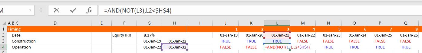
After looking at the layout, put in the dates at the top of the file. Use the EIS (in french you can find the series in the main menu and find the short-cut with the series you can go to the short cut page by clicking on this link. In English (ALT, H, FI, S). Enter the dates as illustrated in the formula the little screenshot below. I used EDATE (in french this is something like DATE.MOIS). If you have the generic macro file open, you can then use SHIFT, CNTL, R to copy the dates to the right. Note that the screenshot has nicer colours because of using CNTL, ALT, C in with the Generic Macro file open. Once you have the dates you should enter the switches (you can call these masks or flags and you can use 1,0 or TRUE, FALSE). Use the SHIFT, CNTL, R to copy to the right. To summarise, put the numbers of the period at the top. Then link the very first date to the financial close. In the cell to the right, use the EDATE function and press SHIFT, CNTL, R. Below the dates put a construction and operation switch. You can put the start and end dates to the left to document what you are doing. For the construction period, the dates at the left are the financial close date and the commercial operation date. For the operation period, use the commercial operation in the left most column and use the decommissioning data in column H. Once you have the dates, use the AND function (E in french). You always refer to the date line in row 2. For example, for the construction switch use the formula AND(date>= FC date,date<COD). For the operation flag or switch, the formula is AND(date>=COD,date<DECOM).
Part 3: EBITDA and Project IRR
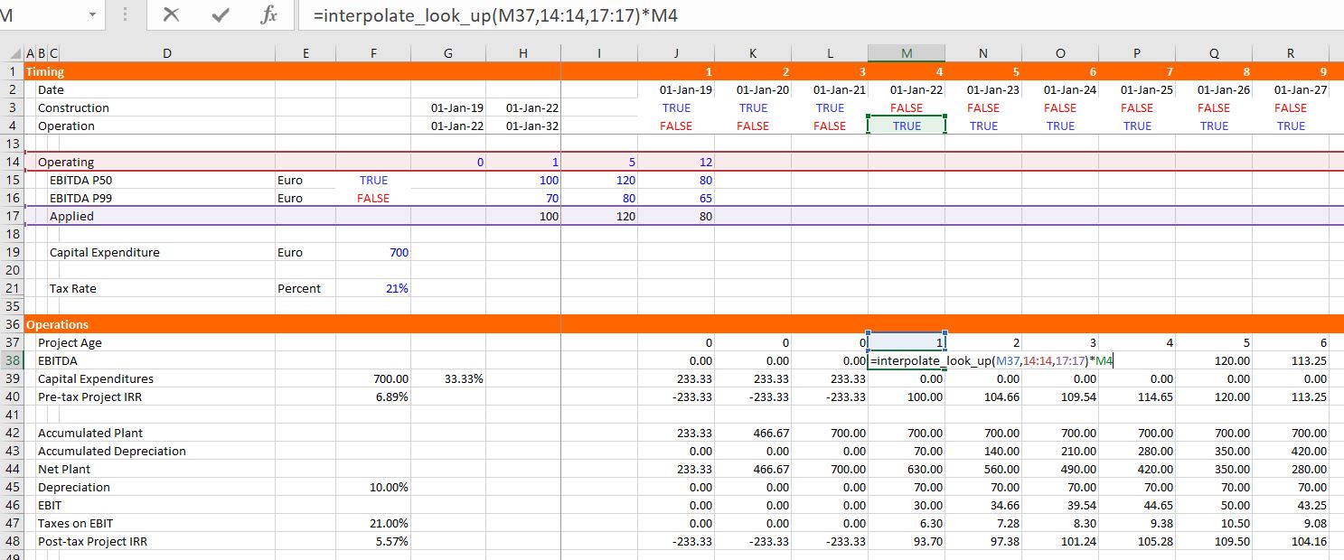
One thing that may be a little tricky in the model is to compute the EBITDA from either the P50 or the P90. The calculations of EBITDA are displayed in the screenshot below. You can use the TRUE and FALSE inputs in column H to chose which scenario is in place (the false in cell H16 is NOT(H15)). In the screenshot below, the numbers in line 17 are computed with the TRUE and FALSE. To implement either the P50 or the P90, you go to line 17 and multiply the numbers in the P50 line (line 15) by the TRUE or FALSE in column H and you do the same with line 16 for the P90. The formula for line 17 is: TRUE * Line 15 + FALSE * Line 16, where the TRUE or FALSE come from the items in column H. Then, the idea is to interpolate the EBITDA rather than using a step function that you can compute with LOOKUP (RECHERCH in french). You can see how the LOOKUP function works by going to the associated link. Then you can try to interpolate the EBITDA numbers instead of using the LOOKUP function. To do this you should try to use the INTERPOLATE LOOKUP function that I created and that you have to bring into your file (the link is provided to retrieve this function with instructions on how to upload the function). The manner in which you can compute the EBITDA from a counter and the INTERPOLATE function is shown in the screenshot below. You should make the counter by accumulating the operating switch. Then you should use the entire row with the LOOKUP or INTERPOLATE LOOKUP function. (If you are having trouble bringing in the INTERPOLATE function, use the LOOKUP function and model EBITDA as a step function). The LOOKUP function starts with one input that corresponds to the item that is being looked up — it is typically a date or a counter. To implement LOOKUP or INTERPOLATE, you then put in the entire row for the corresponding item — in the case below, this is line 14. Then you click on the entire line 17 that will arrange the EBITDA. Finally you should multiply the INTERPOLATE formula by the TRUE or FALSE for the operating switch as is shown on the screenshot. Use the SHIFT, CNTL, R to copy to the right. (Notice how there is a freeze pane for the dates and the switches). I think it is worth giving up completely on VLOOKUP or HLOOKUP (in french RECHERCHV or RECHERCHH). After you have created the EBITDA, the rest of this portion of the model to compute the pre-tax project IRR and the post-tax IRR (TRI in french). Pre-tax IRR is computed from pre-tax cash flow which is EBITDA less Capital Expenditure. Then compute depreciation expense and use the depreciation expense to compute EBIT. With the EBIT you can compute the operating taxes and the after-tax cash flow.
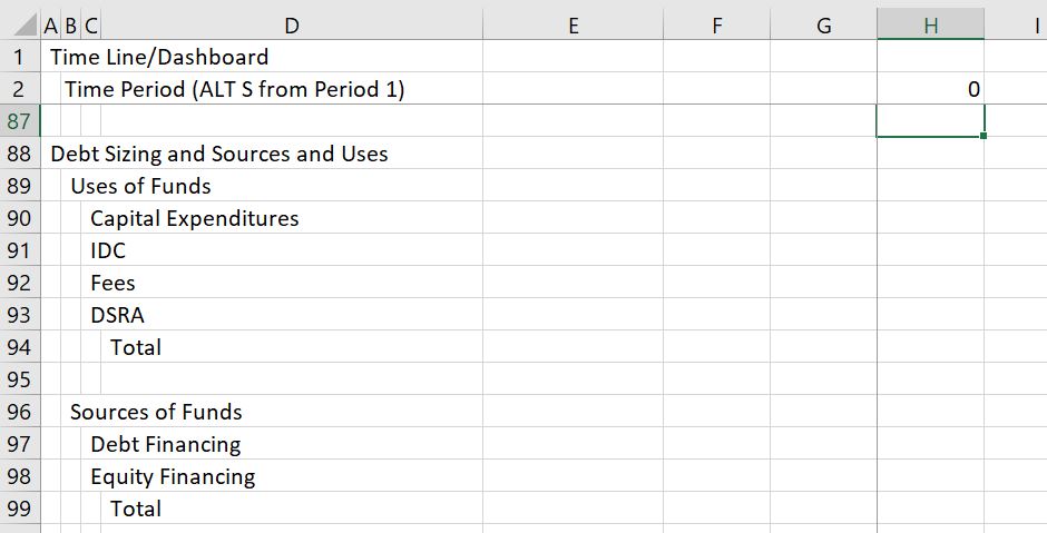
Part 4: Summary Sources and Uses and Debt Size from Sculpting
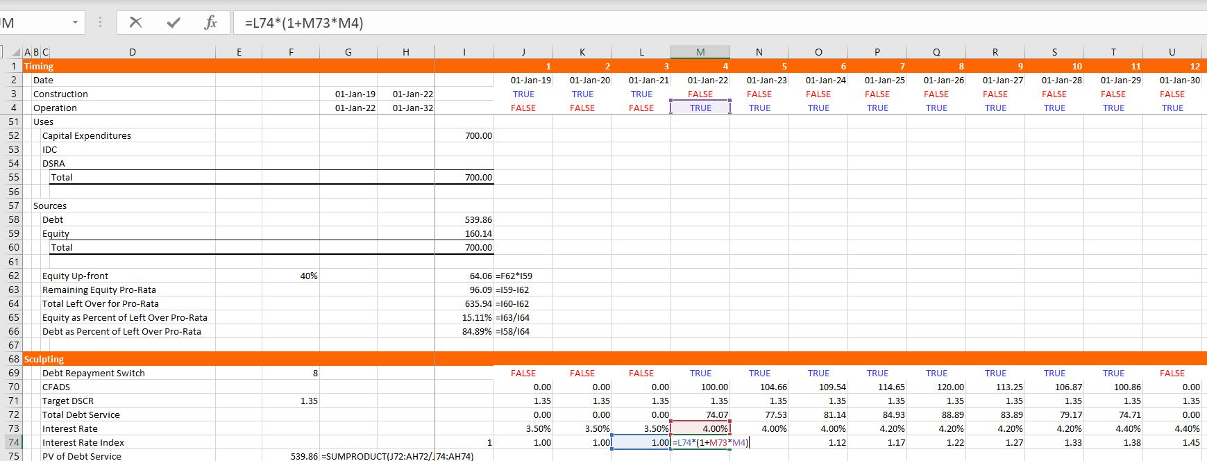
The next step of the model is to set-up a summary sources and uses of funds statement and a sculpting schedule to evaluate the the debt size. In this case, assume that the size of the debt is driven by the minimum DSCR and the minimum DSCR is applied for each period. You can fill in the sources and uses except for debt items which is very simple — just sum up the capital expenditures and compute the equity as the total cost less the debt. To find the debt size from sculpting, you can go to the sculpting section just below the sources and uses as shown in the screenshot below. For now, fill in the CFADS line with the EBITDA instead of CFADS (which is of course not correct). Use the SHIFT, CNTL, R to copy to the right. You should also multiply the CFADS by a debt switch that contains a TRUE in the periods of the debt repayment. Then compute the debt service as the CFADS divided by the DSCR and apply the SUMPRODUCT with and interest rate index in computing the NPV of debt service which is the the size of the debt. If you want some more background on basic sculpting, go to the associated link. Note that you should make sure that the DSCR is working with the TRUE and FALSE for the P90 or the P50 DSCR in the assumptions section. Once you put the debt amount from the PV of the debt service into the sources and uses, you can work on the pro-rata percentages used for computing period by period funding. Pro-rata percentages compute a pro-rata base that is the non-up-front equity plus the debt (note that all of these numbers must be reduced by the capitalised interest). I hope you see how useful it is to have a summary sources and uses of funds.
Part 5: Funding During Construction Cash Flow Statement
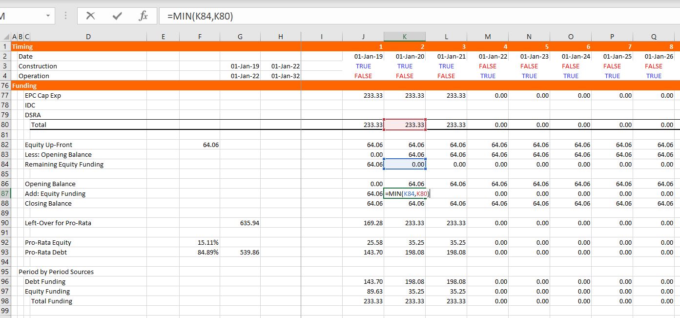
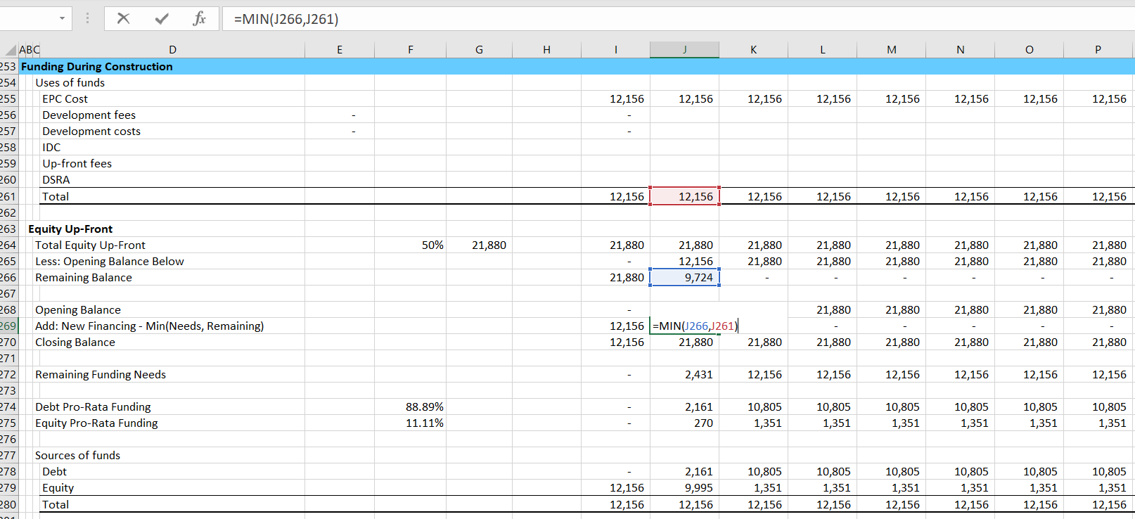
A project finance model has two cash flow statements. You probably know the cash flow waterfall after construction that occurs after the COD. The other cash flow is the cash flow statement before the COD that works through how much funding is required and where the money comes from. The screenshot below illustrates the funding section. Begin with the same titles that are in the uses of funds including the EPC cost, the IDC and so forth. Fill in the items on a period by period basis. Then begin with the up-front equity. To model how much up-front equity can be used I suggest setting up a little table that evaluates how much remaining up-front equity must be used before pro-rata funding kicks-in. Once you have this table you can compute the up-front equity funding using the MIN function as shown in the screenshot below. The MIN function is MIN(Funding Needs, Remaining Funding). After the up-front funding, you can enter the pro-rata percentages to the left and then compute the funding from equity and debt pro-rata funding. These percentages which are shown in the screenshot below come from the summary sources and uses analysis.
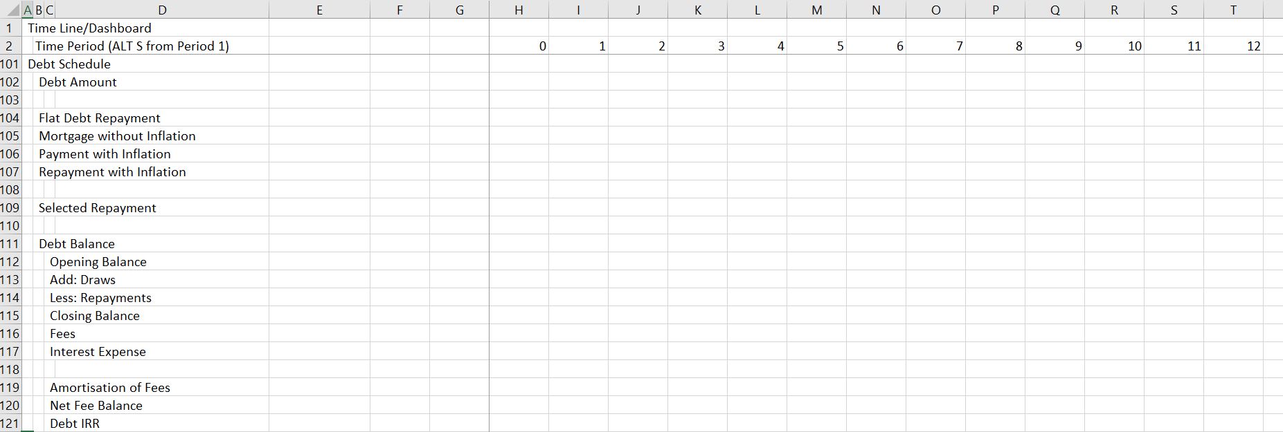
Part 6: Debt Schedule and DSRA Schedule
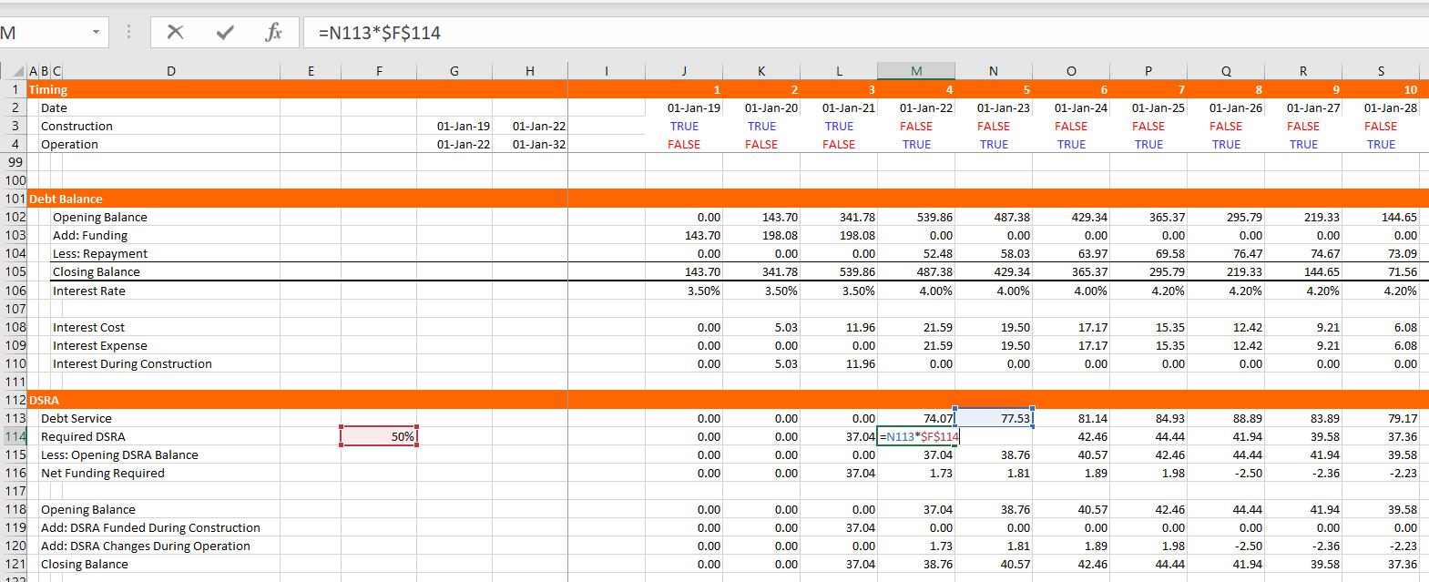
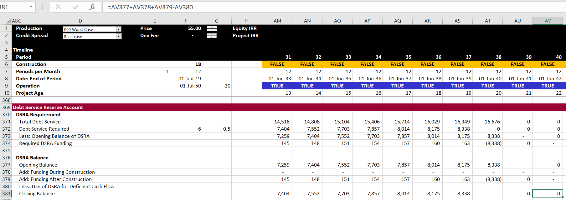
With the funding defined and the sculpting defined, you are ready for the debt schedule which keeps track of debt balances and derives interest expenses. To keep things less tedious, fees are not included in this example which is illustrated in the screenshot below. Once the debt schedule is complete, you can use the debt service to compute the required DSRA balance and the DSRA account. The debt schedule is pretty standard with the opening and closing balance, repayment and interest. In order to compute the repayment, just use the idea the debt service is equal to interest plus repayment which means repayment is debt service minus interest. Then you can go to the debt service line and subtract the interest from the bottom of the debt balance. With the debt balance you can compute the DSRA. You can take the pain out of computing the DSRA by starting with the required DSRA at the top of the section. This required DSRA is the debt service from the debt schedule in the subsequent year multiplied by the DSRA percent. Then, when you have the required DSRA, you can subtract the amount already in the DSRA (the opening balance of the account). Once you have the required amount of the DSRA, put in an opening can closing balance and add the required funding. But when you add the required funding (which will eventually be negative), you should split it between funding during construction and funding during operation (which will eventually be negative). To do this, multiply the required funding by the operating switch or the construction switch.
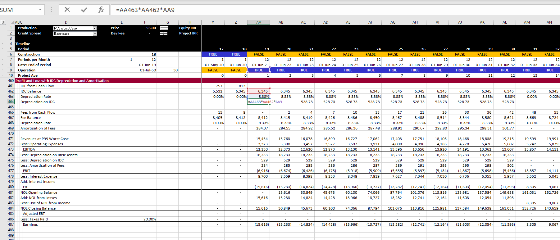
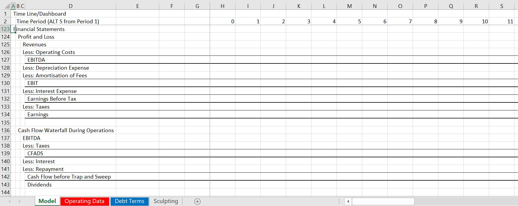
Part 7: IDC Depreciation and Profit and Loss
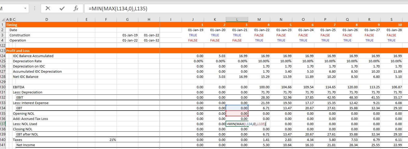
CFADS is computed as EBITDA less taxes which means that you need to compute taxes and, in turn, you need to work through a profit and loss statement. You already have EBITDA, interest, and a tax rate from other items in the model, but the depreciation expense must be adjusted for IDC. So, in the screenshot below, you can see that I put IDC depreciation at the top of the P&L. This is not very conventional, but I do this to illustrate the flow of the model and the fact that IDC deprecation cannot be computed until after the debt schedule is computed. To compute IDC depreciation, accumulate the IDC, use the depreciation rate from the basic deprecation calculation above and compute the accumulated depreciation. Next, you can work through the income statement and get to the tax page. In computing taxes, there may be a net operating loss. The NOL can be computed by setting up a balance account and increasing the NOL when the EBT is negative. This can be accomplished by using MAX(-EBT,0). The NOL is used when the EBT is positive and the opening NOL balance is positive. This can be modelled using MIN(MAX(EBT,0),Opening Balance) as shown in the screenshot. Once you have the additions to the NOL and subtractions from the NOL, you can compute an adjusted EBT calculation and the taxes paid. The adjusted EBT is the EBT before the NOL plus the addition to the NOL, minus the use of the NOL.
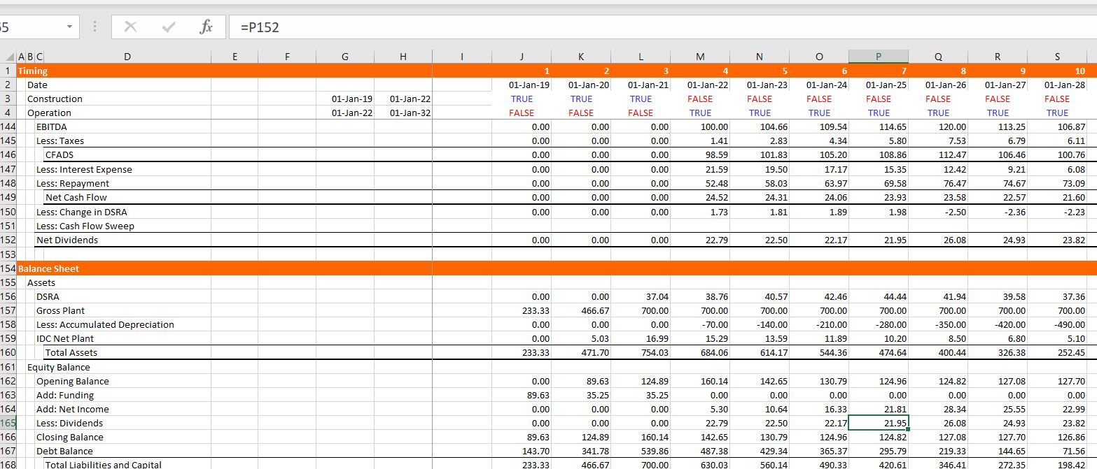
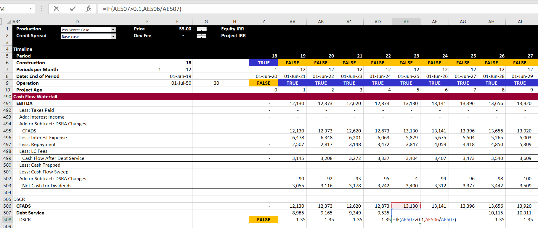
Part 8: Cash Flow Waterfall and Balance Sheet
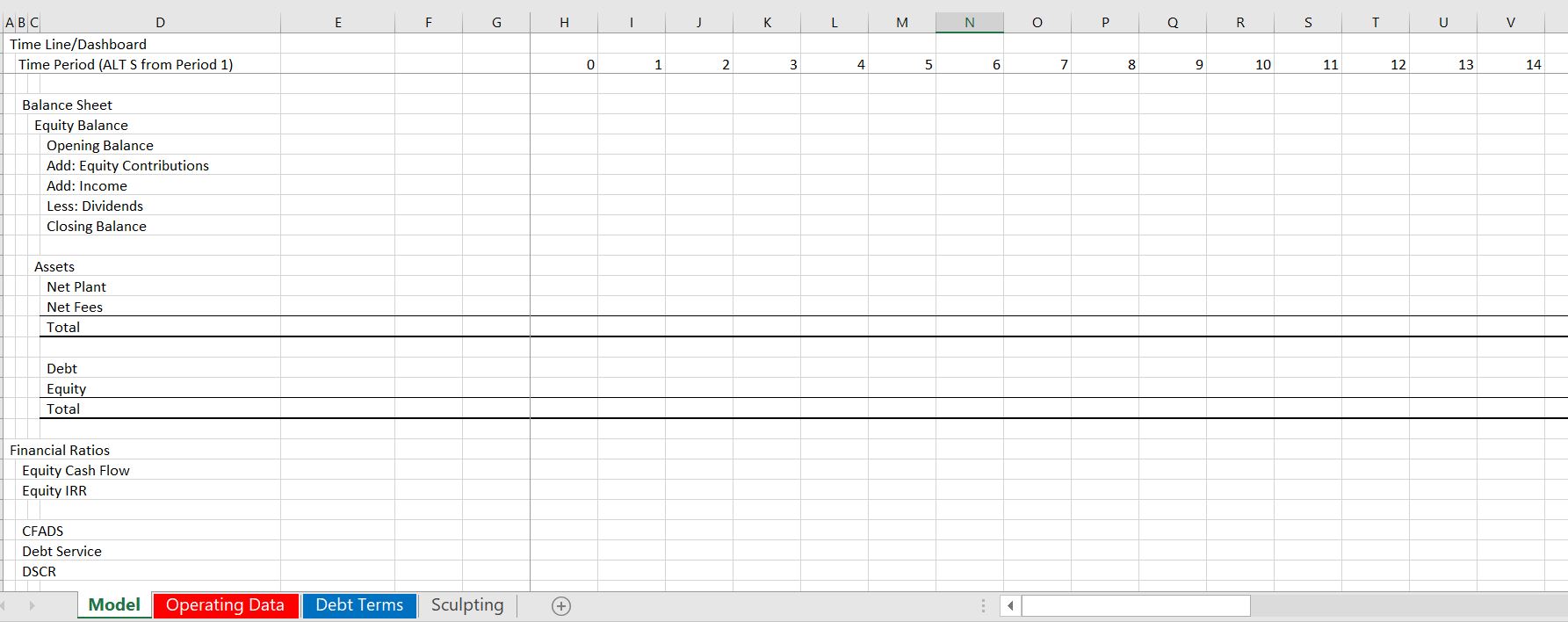
We are finally just about finished with the model, we just need the cash flow statement and the balance sheet. With one exception, these two statements involve just finding other rows, linking the formulas and then computing a few sub-totals as shown in the screenshot below. For the cash flow statement, just start by linking the EBITDA, the taxes, the interest expense, and the repayments. In constructing the balance sheet, just go up and find the closing balances of various accounts like the plant balance, the accumulated depreciation, the debt and the IDC plant balance. The exception is computation of common equity. For common equity set-up an account with the opening and closing balance. Add the funding which is the last line of the funding cash flow statement; add the income which is the last line of the profit and loss statement; and, subtract the dividends which is the last line of the cash flow waterfall as shown in the screenshot. When you do this, the balance sheet does not balance. This is because the IDC from the debt balance has not been attached to the funding statement and the DSRA funding has not been attached and the sum of the IDC funding requirements and the DSRA funding requirements are not in the summary sources and uses statement.
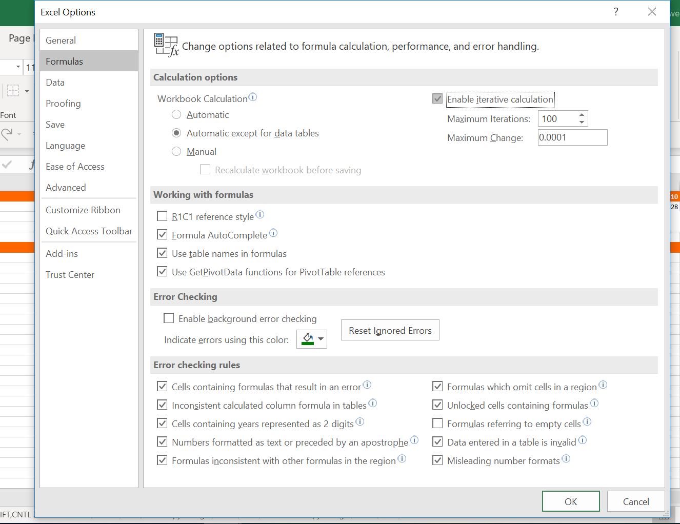
Part 9: Circular References and Iteration
It is really painful for me to suggest this, but to finish this part of the model can you use the iteration button in excel. The screenshot below shows you how to do this, but I really hope you will hardly ever use it. I explain elsewhere that when you put in a bad input; when you make a mistake; when you try to use the goal seek, your model blows up. But let’s go anyway and then see what happens when you make these errors. First go to the IDC line in the funding section and fill in the amount from the interest during construction in the debt. Then stay in the funding section and go to the DSRA. You can attach this line to the line with the DSRA funding during construction. Next, continue going backwards and put the sum of the IDC from the funding section into the sources and uses summary. Do the same for the sum of the DSRA function, namely put the sum of the DSRA line in the funding section into the summary sources and uses. Finally, go to the sculpting section and replace the EBITDA that we used with the CFADS line way down in the cash flow statement. Once you do this, the balance sheet should balance. Finally compute the DSCR and the equity IRR. The sDSCR should be the same as the target. To compute the equity cash flow, you can look up in the balance sheet and find the equity funding and the dividends. The dividends are positive cash and the equity funding is negative.
In this final section I will show you a couple of problems with using the iteration button. First you must save the file. Next make an error in the input. Put the letter a in the DSCR. You will get a bunch of errors in the model. Then press CNTL Z to undo. This does not clear the errors. Now delete the debt service row in the sculpting section (after re-opening the model) – use CNTL – and remove the row. This time you will get a bunch of #REF’s. Try to undo again and it still does not work. So, you better close the file and re-open it again. Now try to use the goal seek. Why don’t you set the IRR to 10% by changing the last EBITDA. The goal seek just goes around and around and does not work.
The button below has the completed file. You can check your work or just look through the file.
Section 7: Modelling More Complex Situations with Multiple Debt Issues, Sculpting and Unavoidable Circular References

Setting-up Debt Assumptions and Debt Schedules
I have taken a long time to add the debt issues to this A-Z lesson. When you add debt to a project finance model you will run into circular reference issues. These circular references come from both funding and and repayment issues. In working through the various debt structure subjects I show how to set-up the model without circular references. Then, in the next section, I show you how to use UDF’s which will enable you to check your work and to create nice flexible dashboards. I hope you will stop being a copy and paster in all areas of your life.
Before starting to go though the various mechanical debt financing subjects, you should download the two files that I am using for this exercise. I am sorry, but these files are different from the files above as I have tried to focus on tricky debt sizing issues. These file connected to the buttons below use the case of a wind farm with different debt sizing possibilities (from P99, P50 and debt to capital), multiple debt sizing issues and multiple re-financing possibilities. You can download the files that are used for completing exercises and a completed version of the files by clicking on the buttons below.
Videos on Debt Structuring
Structure of Inputs and Assumptions
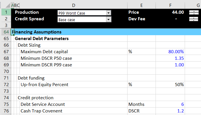
The manner in which you can set-up assumptions when you have multiple debt issues is illustrated in the screenshot below. You should understand that some parameters apply to all debt issues. You cannot have more than one overall debt service coverage ratio (you can have a senior DSCR and a total DSCR — not a subordinated DSCR). You cannot not have more than one overall debt to capital ratio. The DSRA that protects lenders is generally on the overall debt service. Other parameters such as the interest rate, the debt tenure and the repayment pattern of debt can be defined on an individual debt issue basis. The screenshot below illustrates how you can set up the debt assumptions with one debt issue. The first screenshot illustrates how there can be multiple overall debt sizing constraints and how the the funding of debt is driven by a parameter for up-front equity funding.
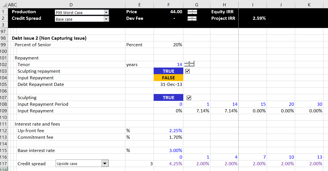
The screenshot below illustrates inputs and assumptions that should be input on an issue by issue basis. The first input is for the percent of the total debt that is represented by the debt issue. I have labeled this issue as a not capture issue. This is because if there are multiple debt issues and sculpting, there must be one issue that captures the rest of the debt service and assures that the total debt service is met. I find the whole idea of sculpting for multiple debt issues complex and there I have included a separate page that deals with the multiple debt issue sculpting subject. The debt tenure is entered by issue and if the debt with the longest tenure should generally be the debt capture issue. You can enter a grace period near the tenure and you can put in specific dates for the start and end of the repayment. Note that I have used the generic macros file to colour the various things (please just try this). As with my general philosophy I hope you keep the structuring of the debt issues consistent — the size, the funding, the repayment, the interest rate and fee and the protections.
Structure of Debt Size and Summary Sources and Uses of Funds
Once the inputs are established, I suggest structuring the whole model without circular references, meaning that you enter the titles and make various calculations. Structuring the whole model without the circular references means that you can leave some items like IDC in the periodic sources and uses funds blank. You may also make some errors on purpose like not subtracting taxes in computing CFADS In other cases, like for the debt IRR, you may want to just enter a fixed number.
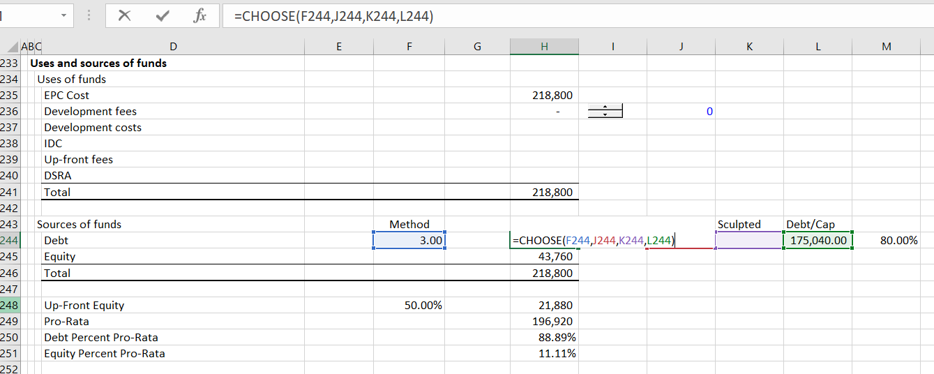
Now let’s move to the modelling of debt size, debt funding, debt repayment, interest and fee costs, and credit protections. One way or another I suggest that you put in a summary sources and uses of funds statement with the total amount over the construction period. If you are setting up your model, you will not be able to enter the IDC (I Don’t Care, or interest during construction), the DSRA, and the fees. You will generally also not be able to enter the amount of the debt. But just enter a placeholder for the debt and leave the IDC, DSRA and fees blank. Then your summary sources and uses of funds should look something like the screenshot below. This is the first step of the analysis and this is related to the debt sizing. Note how I have put options for debt sizing from debt to capital or from input debt or from sculpting to the right of the debt amount and these are not yet filled-in. The fact that these items are not entered yet should be giving you anxiety about circular references. When you have to go downstairs to find stuff, circular references are an issue.
Cash Flow Statement Number 1 – Sources and Uses During Construction
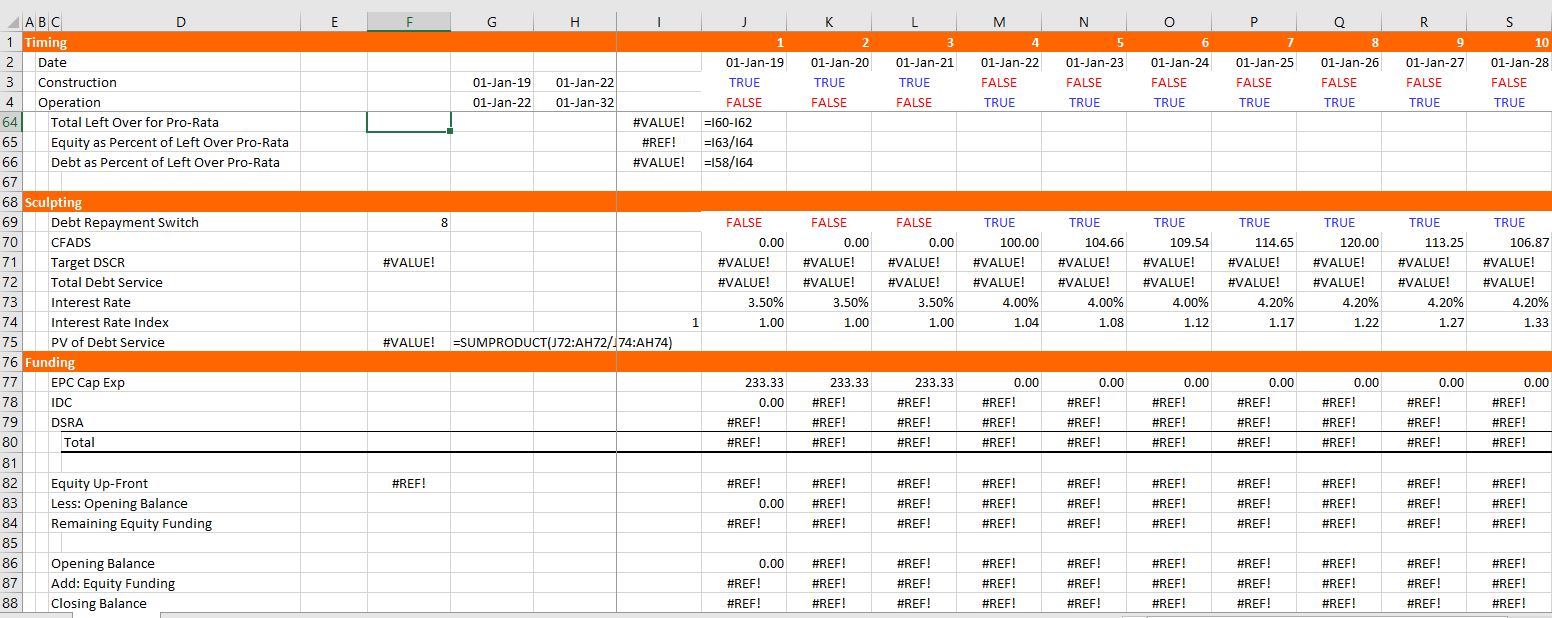
Now let’s turn to funding of the debt during construction given the amount of debt and equity from the summary sources and uses of funds statement. I am using the Hedieh method of entering the equity up-front as an input variable. I think this is brilliant. If you want everything to be pro-rata, you can enter zero as the equity up-front percent. If you want to use all up-front funding, you can enter 100% for the input. Of course you can enter anything between. Given this input for which I used 50%, which implies that some of the funding is equity up-front and some is pro-rata. In the screenshot above, in the section below the sources and uses of funds I have computed the percent of funding that comes from pro-rata debt and pro-rata equity. To make this calculation compute the 50% of equity up-front first. Then you can derive the total pro-rata funding. The debt percent of pro-rata is the total debt divided by the pro-rata funding and the equity is the remainder.
Once you have the pro-rata percentages you can enter the sources and uses funds statement on a period by period basis. You should think of this as a cash flow statement before COD. Before COD there is no EBITDA and no cash inflow, so everything is about finding cash to fund the various needs which include capital expenditures and can include IDC, fees, DSRA funding, Development costs, Development fees and so forth. An example of cash flow statement before COD (the sources and uses of funds) is illustrated in the screenshot below. Note that the numbers are not filled-in. This is again because of the circular reference nightmare.
To compute either equity-up front or pro-rata funding, you can begin by evaluating the equity up-front. I have seen many ways to do this, but I start by computing the amount of remaining equity that can be used to fund equity that will be used in the MIN function. I do this by first computing the total equity commitment an then subtract the amount of equity already used which is the opening balance. Then, I compute the opening and closing balance of the equity. The amount of funding is computed with the MIN function where you compute the minimum of the funding needs or the remaining equity.
Equity Funding = MIN(Remaining Funding, Cash Needs)
Structure of Debt Schedules with Multiple Issues
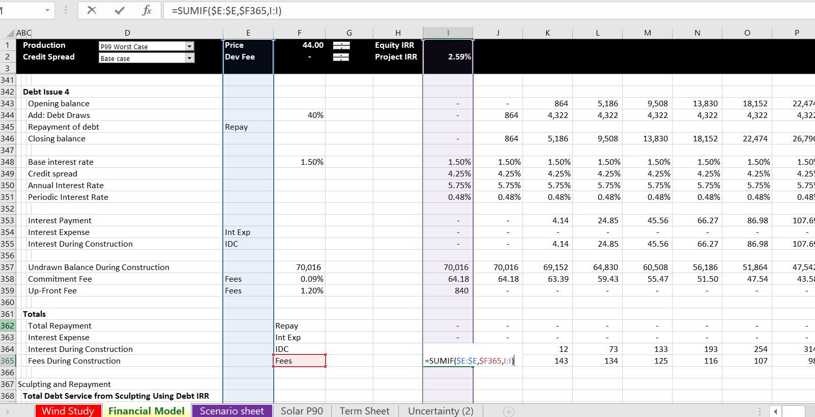
After the first cash flow statement — the sources and uses of funds by period — is established, you can enter the debt schedule. The debt schedule simply presents the opening balance, additions and closing balance. I cannot imagine a project finance model that does not have a debt schedule. In the example below, I have left out the repayment which is addressed in the next section. As you can see, the debt schedule also includes interest rates and fees with a separation of interest between IDC and interest expense. This is pretty standard with maybe the exception that the debt draws are computed from the percent of total debt that is gathered from the sources and uses of funds statement.
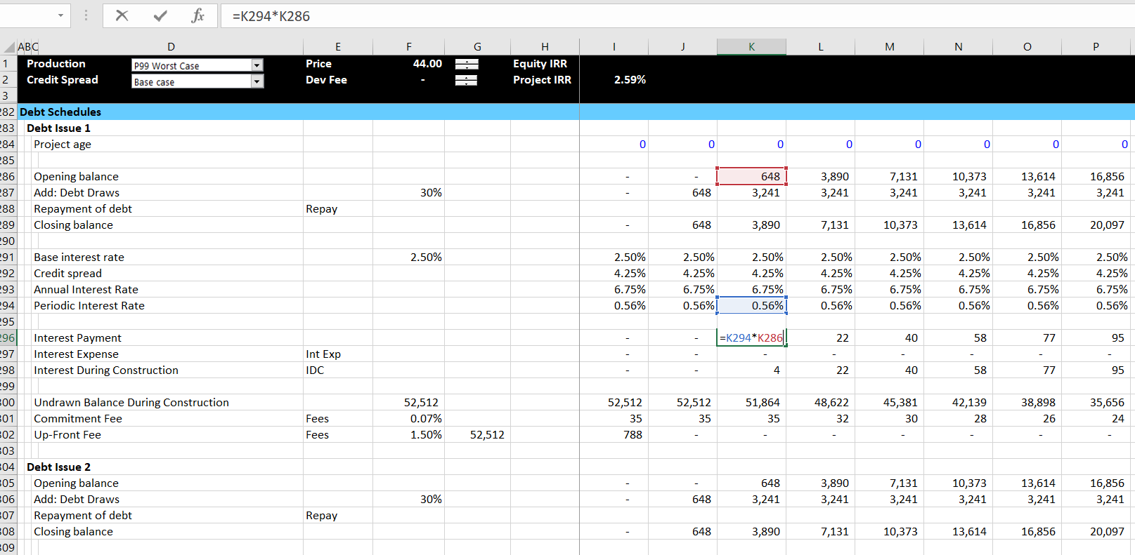
I have also included a screenshot with the summary of all of the debt issues below. This just adds up all of the interest cost and the IDC and the fees using a SUMIF function. Of course I apply the lazy principle and use the SUMIF with the entire columns of data. As with the debt schedule, this is just a long and painful process. Note that after the total fees and the total IDC is computed, I have not placed the amount in the sources and uses of funds. When you put the IDC and the fees into the sources and uses of funds, a dreaded circular reference occurs.
Structure of Repayment with Multiple Sculpting
In this A-Z exercise I have included repayment schedules where multiple debt issues are used to sculpt. On another page in the advanced project finance section I explain this process in detail. Please note that you can compute this by temporarily pretending that CFADS is the same as EBITDA. You will change this when you implement the UDF below. In brief, if you want multiple sculpted issues that produce both the target DSCR and the correct allocation of debt, you can do the following:
1. Compute the aggregate amount of debt with the aggregate CFADS using a debt IRR. To compute the debt IRR you will have a circular reference because the amount of aggregate debt is used to apportion the debt, compute debt service and ultimately arrive at the debt IRR itself.
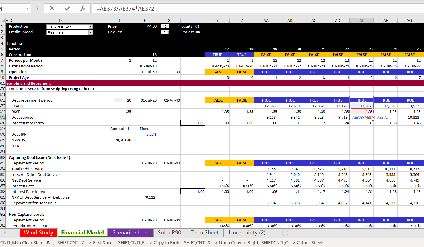
2. Compute the debt service for the capturing debt issue. This capturing debt issue is computed similar to the aggregate debt, but the interest rate on the debt issue is used and the debt service on the other issues are subtracted. The screenshot below illustrates computation of the capturing debt issue and the aggregate debt.
3. Compute the LLCR for the non-capture debt issues. Do this by first computing the debt balance associated with the debt issue where the balance is the total amount of the debt from the NPV of the aggregate debt service in step 1. This is multiplied by the target debt percent. Once you have the debt balance for the non-captured issues, this is the denominator of the LLCR used for sculpting. The numerator is the PV of CFADS at the relevant interest rate. The LLCR that is shown in the second screenshot is computed using the formula:
LLCR = NPV(CFADS)/Debt from Aggregate Debt Balance * Percent Debt
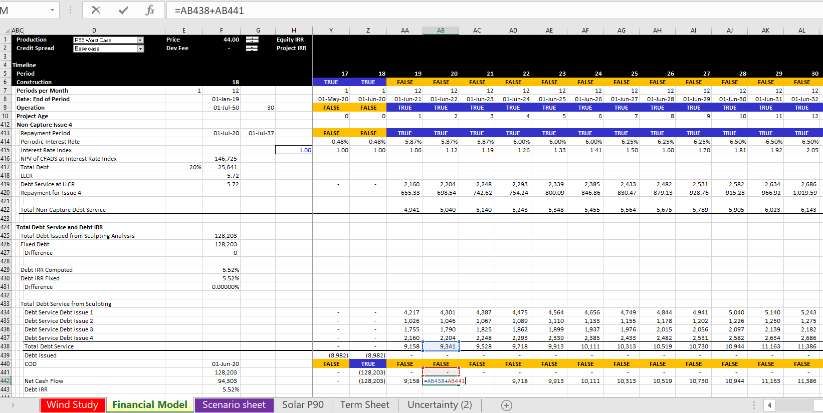
4. The final part involves computing the debt IRR from the total debt service. To calculate this, add the debt service from the different issues. Then put the total debt issued at the COD as the negative investment. With the cash flow on debt, compute the debt IRR. Note that there are two circular references from this process. The first is the IRR and the second is the debt balance. We are setting-up the schedules so do not worry about these yet.
Structure of DSRA Account
The DSRA account can be structured once the debt service is established from the debt schedule. I used to get very worried about the DSRA and the circular references. I have gotten over this fear by beginning with the structure of the DSRA that is illustrated below. Always start with the debt service and then derive the required debt service reserve account. This is illustrated in the screenshot below. I often use the OFFSET function, but I just used 1/2 of the next year’s debt service in this case. If you are using the OFFSET function, use adjust the column with a negative sign for the periods that you want to move from the future as illustrated below:
Debt Service Requirement = OFFSET(Debt Service, 0, – DSRA Periods)
In the above formula, the zero in the middle means that you do not adjust the rows. After you have established the amount of required reserve, compute the amount of required funding or allowed extinguishment. This is the total requirement less the opening balance of the DSRA account. Finally, after computing the required reserve, compute the balance of the DSRA account. This is a normal account with an opening and closing balance. When computing the required funding, separate the funding between the funding during construction which will go into the sources and uses of funds (cash flow statement 1) and into the cash flow waterfall (cash flow statement 2). This funding can be split using TRUE and FALSE switches.
In the screenshot I have not included interest income, the possibility of using a letter of credit instead of a cash DSRA and finally, letter of credit fees. These issues can be painful, especially from the perspective of circular references. I have included these issues in the advanced project finance modelling section.
Profit and Loss Statement with IDC and Fee Depreciation and Amortisation
After you have finished the debt parts of the model you need to go around an compute the CFADS. The difficult issue in computing CFADS is that taxes, interest income are part of the CFADS calculation. But these items depend on the debt which in turn depends on the CFADS. There can also be an issue with changes in the DSRA which can potentially affect the CFADS and is driven by DSRA and debt. When setting-up the model to get ready for the circular reference, you should go all the way to the cash flow statement where CFADS is computed. This requires computation of taxes in a profit and loss statement and setting-up a cash flow waterfall (cash flow statement number 2).
In structuring the profit and loss statement you must include some kind of amortisation or depreciation on financing elements that have been capitalised. I insist that you keep the depreciation expense is separated between amounts that are finance related and base amounts that are associated with capital expenditures, development costs and other items. The base depreciation is necessary for computing the operating taxes and if you mix up the IDC depreciation that is influenced by financing, your project IRR will be wrong. Therefore, I suggest putting the depreciation on IDC and fees near the profit and loss statement where you will compute the taxes paid after financing. This is illustrated in the screenshot below where depreciation rate on IDC and fees is assumed to be the same as the depreciation rate on base assets.
The rest of the profit and loss statement is standard as shown in the screenshot below. The IDC depreciation and the fee amortisation are included as separate items. As in so many other models, the a net operating loss is computed with MIN and MAX functions. The MAX function is used to test whether the EBT is positive or negative. The MIN function is used to test whether the balance of the NOL can be used when there are positive taxes. The one thing that this does not have is expiration of NOL’s. This is a difficult problem addressed in the corporate finance section of the website.
Cash Flow Waterfall and DSCR Calculation
The final statement that you can develop for the structuring section is the cash flow waterfall and the DSCR calculation. The DSCR should be the same as the DSCR that you entered as an input. To avoid circular references I have made an error on purpose and not subtracted the taxes in computing the CFADS. This is shown in the screenshot below. Note that in the screenshot, the DSCR is the same as the DSCR input. The only confusing thing is where to put the changes in DSRA. I put the change in the DSRA after the CFADS so it does not affect the DSCR and sculpting and debt sizing. I address the issue of either putting the DSRA in the CFADS or as an adjustment to debt service in the advanced section. Now we have to deal with circular references.
Section 9: Using Parallel Model/UDF for Solving Circular References
I have been working on a comprehensive model that resolves all of the items that cause circular references with user defined functions for a few years now. I have used the file to illustrate how you can resolve all circular references and allow you to make effective scenario analysis. You can go to the circular reference section of the website to see how this works. Please see clearly that if you use this method, you can just add the parallel model in minutes.
Addition of Parallel Model
Modelling of Debt at P99 and Tariffs at P50
Section 10: Structuring Mezzanine Debt and Shareholder Loans in the Model
Including mezzanine debt and shareholder loans is mainly a pain. These debt or quasi debt issues affect taxes and add to the circular reference pain. You also may have separate sculpting for the total debt that includes mezzanine debt and model a waterfall. In the case of shareholder debt, you do not want to distort any of the debt statistics, cash sweeps or other debt terms by the shareholder debt. The only effect of the shareholder debt is on the tax and possibly on the project cost because of the recording of IDC on the shareholder debt.
Part 9: Structuring Multiple Re-Financing in the Model
First enter one re-financed issue and make sure it works. Then enter multiple issues with the ability to change assumptions.
It is like you add a sheet to your model and then use the Sum function or any other function that is not related to anything in your model. That is the starting point.
Dislike template models. Try to put everything in the world. But agreed. Put in imaginable things.
Then collect a few inputs that you have a fixed amount for. This is the only connection.
You don’t even have to connect if you want to use the parallel model for checking, for sensitivity analysis and for advanced project finance concepts like sculpting with DSRA, adding balloon payments, re-financing etc.
How many minutes does it take to implement the parallel model.
Some points:
- How to copy the template into your file
- Using the debt schedule to find inputs for debt issues
- Understand where to start and end
- Understand the debug option
- Understand the manual and the CNTL, ALT, F9
- Benefit of spreadsheets starting from visicalc was that you could see everything
Sales Points
- Not just another VBA program
- Not as a Sale Program
- Biggest Point is Circular Reference
- People will Resist
Resistance
- This is magic and a black box
- This is like a password protected macro
- This is just another add-in gimick
- History of UDF
Last thing I wanted to do is to program financial model
Circular reference questions and problems with copy and paste
Implementing the UDF Model
Use of Manual Calculation and CNTL, ALT, F9
Explanation of the debug switch
Copying Debt Issues
Interpretation of Output
Changing the Output Structure
Benefits of Parallel Model and UDF Other Than Circular Reference
- Verify Model
- Consistent Way to Check
- Compute Sculpting Repayment in Complex Situations
- Run Alternative Scenarios
- Evaluate Issues that may be Difficult to Program
- Easy to Read Reports
- See Equations for Difficult Sculpting, DSRA and Other Structuring Issues
Circular Reference Resolution — Let’s say you want to make an analysis with where P90 drives debt size but P50 drives price target.
Anybody who has worked in a serious way on project finance models should know about how much the classic solutions to circular references — copy and paste or iteration button — can ruin a model. The problem with copy and paste macros is that your model is suddenly stopped. No goal seeks. No data tables. No simple spinner buttons for sensitivity. No effective summary pages where people can try different scenarios.
Model Verification
Example of mistakes in model that are difficult to verify
Running Alternative Structuring Options without Programming
Complex Issues that You May Not Want to Program, But Make a Quick Analysis
You can verify the model and then say you want to do some more complex things like:
- Debt Sizing Using Alternative Methods
- Balloon payments
- DSRA as L/C with fees
- DSRA moves in CFADS for DSCR calculation
- DSRA moves in Debt Service for DSCR Calculation
- Multiple Issues with Sculpting
- Equity Bridge Loan
- Portion of Equity as Up-Front and Portion as Pro-Rata
- Optimising DSCR for Sculpting with Average Loan Life Constraint and Debt to Capital
Adding/Changing UDF
Put in the output — work backwards
Create a public variable
Construct a model in excel. Can be a simple model
Replicate your excel analysis
By documenting your calculation, you can check it a lot easier
Soon you will realise that it is not much different than making a model; which can be good or bad.
Verification of UDF
Make tests outside of the model
Balance sheet must balance like any model
Debt must be paid off like any model
Check of totals and things like sources and uses
Workings of UDF
Any program (including excel) has inputs, outputs and calculations
These files are from the wikispaces website. I am in the process of uploading all of the files. But in the meantime you can send me an e-mail to edwardbodmer@gmail.com to get the resource library. The files will be located in the project finance section of Chapter 1.
A-Z Part 2 Circular Exercise.xlsm
Circular Mirror Template.xlsm
The third set of videos continue on tricky issues associated with debt. The first video in this set complete the model with no debt and begin adding debt to the models. The last video in this section begins to add a circular resolution template to the model. This is an important idea in project finance where you would like to maintain flexibility in the face of natural circular references.
If you fill in all of the exercises and send me the files along with a small fee, I will publish your name on my website so you can show it to your boss or your future employer. I will also get you an official badge. An illustration of how the models work is shown below. The yellow tabs in the excerpt show the items to fill in. The completed sheets are next to the yellow tabs (I hope I did not make mistakes).
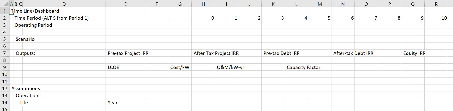
A-Z Exercise with Selected Existing Titles for Solar Model
I was asked to prepare an exercise where people could quickly make a model that evaluates bid prices and other model aspects and can get you most of the result without spending too much time on some of the horrible details that can make project finance modelling so difficult. I was told that making a relatively simple project finance model could not be taught in a single day. This is not true. You can see the essentials of making a model including describing inputs, establishing operating cash flow, computing depreciation and project IRR, incorporating debt, making a cash flow waterfall and computing some key financial ratios in a morning.
The file available for download does this for a simple solar case. To make it really simple I have not even included a construction period and made the model and annual model. For some items I have not included titles so that you can do the really important part of a model which is to structure the model. For other parts, I have included titles so that you do not have to waste a lot of time typing. The exercise hopefully applies some of the fast modelling religion, meaning that it is flexible (except for the one period construction), it is accurate — the balance sheet balances and the debt is paid off; it is structured, where you start with physical operations and then move to revenues, expenses and capital expenditures and then to depreciation which allows you to compute operating taxes and project cash flow. After project cash flow you incorporate debt with a sources and uses of funds statement, and a debt schedule. Only after the debt schedule do you create the financial statements. To download the file, press on the button below.
Part 1: Operating Data
In the first part, you go to the operating data. You use the INDEX function so you can select one of the scenarios. Also put the developer tab in your excel and make a spinner box with the windscreen wiper method to use the form in other sheets. The first part is illustrated in the screenshot below.
Part 2: Timing
In the second part make a timing switch and use the EDATE function (FETCHA.MOIS) to compute the annual dates. I have put some summary outputs at the top of the page. Use the ALT and –> to group the rows and choose to not show the outputs. In English you can use ALT, E, I, S to get the model started for 40 years. With the GENERIC MACROS open, you can use the ALT, S combination. The timing parts of the model are shown on the screenshot below.
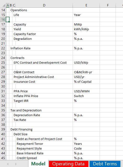
Part 3: Define Inputs
After setting up the time line, pull the relevant inputs from the model from the operating page and from the debt page. The inputs should be discussed and you should see how to change the scenarios with your spinner box. You should understand that the inputs are arranged in a proper order that separates operation from financing; that begins with physical operations; that includes ways to back into the contract price and that includes logical differentiation of the debt parts of the model. When you have linked the outputs, use the CNTL, ALT, C sequence from the GENERIC MACROS to show the location of the inputs and to illustrate the structure of the model. The input section is shown on the screenshot below.
Part 4: Construct the Operations Section of the Model
In the first part of the model I have not provided the titles. You are supposed to get to the volumes produced in MWH which is the basis for revenues. To do this you need to know how much the solar capacity factor or yield will be. I suggest you enter the driver of the formula in a left hand column, that you put in the units in a left hand column and that you use SHIFT, CNTL, R to quickly copy things to the right. You should also compute an index for degradation that begins in year 1 by taking the prior period and multiplying it by (1+degradation). Then you can divide the capacity by degradation and compute the capacity after degradation. You can use whatever method you want to insert the rows. You can create your own short-cut key for the underline.

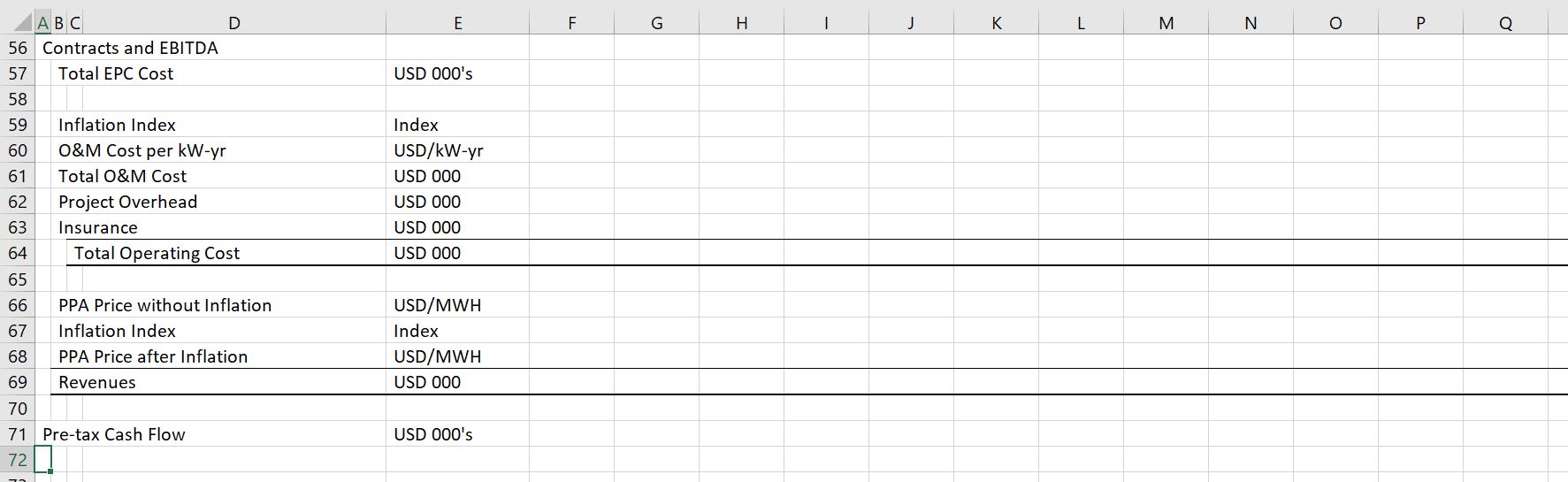
Part 5: Revenues, Expenses, Capital Expenditures and Free Cash Flow
In any corporate finance model, M&A model, real estate model or project finance model, you will need revenues, expenses and capital expenditures. The assumptions that create these three items (along with working capital) will drive all of the rest of the analysis. In the next section you are to compute revenues, expenses and capital expenditures from the inputs. I think it is a really good idea to put the drivers of each formula in a left hand column so you can be transparent (I hate looking around for where the numbers came from). In this part of the analysis I have given you the titles as shown on the screenshot below. Once you have computed the project IRR you can use a goal seek and a macro to evaluate the required price.
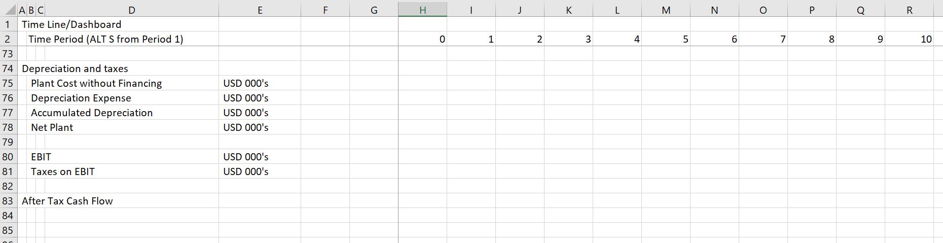
Part 6: Depreciation, Operating Taxes and After Tax Free Cash Flow
If there were no taxes and you did not want to show a profit and loss statement you could eliminate this part of the model. With taxes, the shield from depreciation is an important item. Compute the depreciation by setting up an account with the balance of plant as shown below. When you compute depreciation you can use the MIN function to make sure the depreciation does not exceed the net plant balance. Once you have the depreciation you can compute the EBIT, the taxes on EBIT, the after tax project cash flow and the project IRR. The screenshot below illustrates this part of the model.
Part 7: Sources and Uses Prior to COD
Once you have completed the operating cash flow and operating taxes you can move to incorporating debt in the model. In every project finance model there should be a sources and uses of funds for evaluating cash flows during the construction period. You can think of this as a way to evaluate debt sizing. In the example, you can fill in items on the sources and uses of funds from the inputs and items above the sources and uses. Note that this is not realistic as items such as interest during construction and fees come from below not above and you get a circular reference.
Part 8: Debt Schedule
The debt schedule must have calculations for debt repayment, interest expenses and fees. Repayment is often the most difficult aspect of a model. There are alternative methods demonstrated to compute the repayment including flat repayment, mortgage repayment and inflated repayment that matches the cash flow when inflation is applied in the price. Use the INDEX Function to select one of the three methods of repayment. A screenshot is shown below.
Part 9: Profit and Loss Statement and Cash Flow Statement
Now you are to the easy part. The only reason that an income statement is necessary in a project finance model is to compute taxes and to compute net income for purposes of balancing the balance sheet. The cash flow statement can be more complex if there are cash sweeps, covenants and other items.
Part 10: Balance Sheet and Financial Ratios
The final part of the exercise is to put together a balance sheet and compute a couple of financial ratios. The balance sheet components should all come from items in the model and the equity balance should be computed. Ratios like IRR, DSCR and LLCR come from the cash flow statement.
Exercise that Includes Construction Period
I was asked to prepare an exercise where people could quickly make a model that evaluates bid prices and other model aspects and can get you most of the result without spending too much time on some of the horrible details that can make project finance modelling so difficult. I was told that making a relatively simple project finance model could not be taught in a single day. This is not true. You can see
Excel File with Exercise for Creating Combined Cycle Model with Timing and Construction Issues
Case Study Exercise on How You Can Evaluate and Existing Model
Some unlucky people have to create models and deal with circular references and many horrible details like withholding taxes on four tranches of debt. More people have to interpret and use models that is arguably even more disagreeable because of the way models have become cumbersome and overly detailed.
This case study and exercise is designed so that you can more efficiently evaluate models created by other people including dissecting cash flow in the models, computing alternative financial ratios, adding your own scenario analysis, dissecting the model with sensitivity analysis, creating an summary page the conveys the transaction, making effective graphs the illustrate risks and finally formatting the model with nice colours and titles. My hope is that this exercise will be practical for you and that you can use some of the ideas in your current job immediately.
The file that I have used for this case is the completed case from the above model. But it could be just about any project finance model, corporate model, M&A model or other financial analysis that has a few inputs and outputs. The base model that I have chosen for this exercise is available for download by clicking on the button below.
Introduction to the Model Review Assignment
I have structured this assignment by attempting to explain the details of how to complete the excel stuff. Then I have included questions that should be completed with only one or two sentences where you tell me the implications of the modelling tasks. I have also provided titles for many of the items so that you do not have to waste a lot of time typing stuff and the exercise will not take too much time. I strongly suggest that you do not do this exercise on an Apple computer; that you open and use the GENERIC MACRO file, the LOOKUP INTERPOLATE file and the SCENARIO REPORTER file to make the case go faster. These three files are available for download below.
Part 1: Dissecting Cash flow
Use the SUMIF function to get the data to annual amounts. When you use the SUMIF, click on the entire row. Question – how does the IRR on the project and equity compare to overall stock market returns. Do you think this is realistic.
Part 2: Computing Alternative Financial Ratios
I hope that you learn to look at ratios other than the DSCR. In this case you can examine the LLCR and the PLCR. The only calculation you have to make for this is to use the SUMPRODUCT function below the cash flow statement with the interest rate index and to find the debt at COD from the sources and uses. Explain how to interpret the DSCR, LLCR and PLCR.
Part 3: Adding your Own Scenario Analysis
Use the scenario manager to add a scenario. In this case could you invent a few cases with different inputs. Change the following: the project cost, the life of the plant, the availability. Then open the scenario reporter and create a scenario report.