This page works through time series equations that underlie Monte Carlo simulation and in particular the underlying formulas for mean reversion and other factors. I hope in each page I make it clear that development of the time series equation is far more important than running the simulation using multiple draws from a random distribution. In thinking about risk, an essential concept is the notion that things can go up and down and then come back to the average level — mean reversion. Alternatively, things can keep going up and down without some kind of inherent average. Oil prices follow a mean reverting patter while stock prices are supposed to have no mean reversion. I have been frustrated for many years in attempting to incorporate mean reversion into Monte Carol Simulation. Time series equations must have some kind of stochastic element, but they can include a host of other variables, the most important of which is mean reversion. I try to explain these things with some simple excel equations rather than trying to understand formulas in text books. Factors other than mean reversion can include minimum and maximum conditions that reflect periods of surplus capacity. A basic time series equation can be expanded to include sudden jumps, mean reversion, minimum levels, maximum levels and trends.
The fundamental equation to understand volatility and mean reversion is the notion that when you do not have mean mean reversion, the variance (the square of volatility) increases with time. You may have seen the eqation where you adjust the computed volatility in a day and then convert it to annual volatility. To do this you can use the square root of time as illustrated below. (I never understood why you take the square root of time until I messed around with Monte Carlo simulation). The formula to convert daily volatility to annual volatlity assuming 252 days trading days in a year is:
Annual Volatilty = Daily Volatility x (252) ^ .5
Annual Volatility = Daily Volatility x (Periods in Year) ^ .5
Annual Variance = Daily Variance x Periods
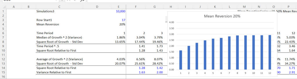
This means that if you compute the variance as the percent change in the output from period to period over a simulated period, for example Pt/Pt-1 -1 or LN (Pt/Pt-1) then the variance should be the square of the volatility input. But when you compute LN(Pt/Pt-2) the variance should be 2 times the volatility input or the volatility should be 2 ^ .5 times the volatilty input. If you go out to 252 periods, the volatilty should be 252 ^ .5 or 15.8 times the volatility input. If you go out two years instead of one year then you would multiply the 504 ^ .5 to compute the second year volatilty. This means the volatility of the simulation LN(Pt/Pt-504) should be 22 times the volatiltiy computed from one period. In the files below I demonstrate that this does happen with a non-mean reverting time series.
In studying prices, there seem to be very few things — even stock prices — that follow this kind of pattern where the variance continues to increase over time. Other series like oil prices, gas prices and other commodity prices clearly follow a pattern where the standard deviation does not increase with the square root of time. This equation is the key to test whether mean reversion really exists and then to make adjustments for mean reversion. Specifically, if there is mean reversion, then the standard deviation used to compute annual or monthly volatility will be less than the standard deviation computed with the formula Annual volatility = Periodic Volatility x (periods per year) ^ .5.
.
The notion of making equations can be relate to philosophic ideas. In your life there will be random events such as pandemics, economic recessions, medical emergencies, dog bites, political upheaval … Your task in life is to manage these uncertain events and have a reasonably satisfying life. You can try to get some mean reversion with an education, an open mind, different debt levels and other equations on top of the random events. For example, if you lose your job during a recession but you have watched a lot of videos and have a resilient personality, you have more mean reversion. Maybe you should think about Monte Carlo and time series equations as more of a philosophy than some kind of practical statistical analysis that you will be able to use.
When I first saw Monte Carlo simulation, I was really excited. It wanted to add it to all sorts of financial models and show off how you could incorporate quantification of real options into valuation. But the more I worked on models, the more I realized that it did not seem to be useful in real problems. I now have come around a little to use Monte Carlo simulation to illustrate problems related to credit analysis and some real options issues. For example, you can use Monte Carlo to show derive the acceptable level of the DSCR. When developing a Monte Carlo simulation, it is easy to see how things work if your time series follow a random walk or Brownian motion. But the conclusions are dramatically different if the economic series follows a mean reverting process like most things in the world. I am very frustrated with the manner in which you are supposed to compute the mean reversion parameter and I suggest a method where you use Monte Carlo simulation with alternative mean reversion parameters to derive the appropriate value.
Volatility and Standard Deviation of Rate of Return
Mean reversion is a crucial factor in developing time series. Efficient markets theory suggests the stock prices do not have mean reversion because all of the relevant information is supposed to be incorporated in the current price. This suggests that if prices for example change according to a moving average, you could beat the market by simply buying when the stocks go down and then sell when stock go up. If you could do this and ignore the real information that is changing the value of stocks, the market would not be efficient.
Efficient markets without mean reversion can be modelled by computing the standard deviation of the rate of return. Remember that growth and and rate of return are similar concepts and the standard deviation of the rate of growth is essentially the same as the standard deviation of the rate of return. I wish I would have learnt about volatility by just understanding that volatility is the standard deviation of returns. The idea of a non-mean reverting series representing an efficient is that you look at the standard deviation of returns rather than the standard deviation of absolute returns. The efficient market returns can be represented by a discrete equation or a continual equation just like any growth or return analysis.
Other time series ranging from the weather to oil prices to interest rates are presumed to have mean reversion. For example, if it is very hot one day and the average for prior years is less, then you can predict that the next day or the next week will not be so hot. For oil prices, there are various changes in demand, supply, political events and other market forces that can push prices up or down. But if prices move below the marginal cost of production, oil producers will stop production and the prices will have a floor. On the other hand if prices are really high, then more production will come into the market and the price increase will be limited. The mean reversion can be modelled with the following formulas:
Price (t) = Price (t-1) x (1 + g)
Price (t) = Price(t-1) x EXP(g)
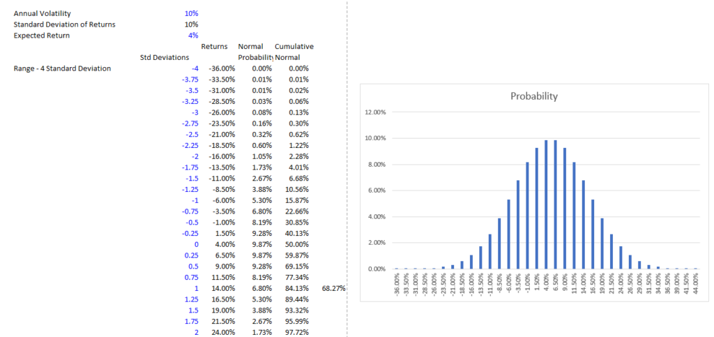
I should be able to tell you that EXP(.05) = 1.05121 (I didn’t know this until I messed around in an excel file). This is the growth rate over a period in really tiny increments where you keep on compounding. In the discrete formula, all of the growth occurs at the end of the year (this is like using the opening balance to compute interest in a debt balance calculation. To see how the normal distribution works with probability, I have made a very simple example where you can plug in the expected return and the standard deviation of return which is the volatility. The range in a normal distribution is about +- 4 standard deviations from the mean. So I make a simple list using EIS and you from -4 to +4 with an increment of .25. Using this you can multiply the standard deviations from the mean by the standard deviation and add the expected return. Then, you can see the distribution of potential returns as a function of the volatility.
When you think of standard deviation you can try to remember the ideas of a normal distribution that only depend on the mean and the standard deviation. I can never really remember if 68% of the predicted values fall between +1 and -1 of the standard deviation. So you can quickly check this in excel.
Price(t) =
Price(t-1) + A x (Mean – Price(t-1) ) +
Volatility x (Price(t-1) x Normsinv(Rand())
When applying this formula, A is the mean reversion factor and it is essential to put the mean price in the equation first and not last. For example, assume that the mean price is 100 and the current price is 150 and A is 20%. In this case you want the next price to go down and not up. So it is important to put the 100 first in the equation which yields 20% x (100-150) or the price moves by 10 back towards the mean. If you are modelling weather with 100% mean reversion from one year to the next, you could put in a mean reversion factor of 100%, meaning the factor would be 100%* (100-150) or -50. In this case it would be better to measure the volatility as the standard deviation divided by the average.
The video below explains how to incorporate various factors of time series equations into an excel model.
[wonderplugin_video iframe=”https://www.youtube.com/watch?v=WliOwYepmHo” videowidth=600 videoheight=400 keepaspectratio=1 videocss=”position:relative;display:block;background-color:#000;overflow:hidden;max-width:100%;margin:0 auto;” playbutton=”http://edbodmer.com/wp-content/plugins/wonderplugin-video-embed/engine/playvideo-64-64-0.png”]
.
[wonderplugin_video iframe=”https://www.youtube.com/watch?v=2mLJEo2ubsw” videowidth=600 videoheight=400 keepaspectratio=1 videocss=”position:relative;display:block;background-color:#000;overflow:hidden;max-width:100%;margin:0 auto;” playbutton=”http://edbodmer.com/wp-content/plugins/wonderplugin-video-embed/engine/playvideo-64-64-0.png”]