On this webpage I demonstrate some mathematics of the IRR and I show that the IRR is just a measurement of the growth rate. I also include discussion of the problem where you cannot compute the IRR for an investment when there is a big change in the sign of the cash flow (which can occur if there is financing with and equity bridge loan that matures after the COD). All the mathematical issues and supposed problems with the IRR come from what to do with cash flows that occur between the initial outflow and the final disposal of the investment — I call these cash flows the middle cash flows. To introduce issues associated with the IRR, I start with a simple example and explain the mechanics of the IRR, the compound growth rate and the NPV. One of the ideas of this page is that you can explain the different statistics with very simple focused examples rather than with a big complex model. The modified IRR (MIRR) is also introduced here and I moan about the problems with the MIRR that just ends up measuring the input re-investment rate. You can find the examples of how the IRR works using the file below. This file includes the examples used in this webpage to illustrate various valuation issues.
.
.
.
Mathematics of XIRR and Compounding
The XIRR converts and hourly discount rate to a daily discount rate through and then discounts using the number of days in a period (this causes a problem with a leap year). If you compute the XIRR and then try and reconcile it to the XNPV, you have to raise the XIRR to the power of 1/365 as illustrated below.
.

.
.

I was just about strangled by a young lawyer a few years ago. She asked me: “What is all of this business with the IRR anyway. What does the IRR mean.” I gave the horrible answer that the IRR is just a discount rate that makes the NPV equal to zero. The lawyer could rightfully have strangled me and said: “does that
.
IRR, Compound Growth and Middle Year Cash Flows
I was just about strangled by a young lawyer a few years ago. She asked me: “What is all of this business with the IRR anyway. What does the IRR mean.” I gave the horrible answer that the IRR is just a discount rate that makes the NPV equal to zero. The lawyer could rightfully have strangled me and said: “does that mean that when every CEO from the president of Apple to a little stock investor thinks to himself, what is the discount rate that makes the discount rate equal to zero when they love investments with a high IRR.” Of course not.
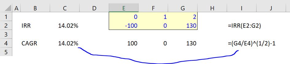
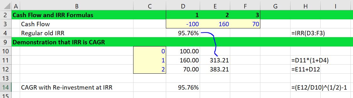
The attractiveness of the IRR is that it measures the growth rate in cash flow. When the stock market grew by 22%, a lot of people got very rich. This growth rate is the IRR. When you make an investment today of 100 and then receive 120 in one year, the IRR is 20% and the growth rate is also 20%. This also works in a situation where you have a multi-year investment. If you invest 100 and get 130 back in two years (like any LBO), the IRR is 14.02% and the compound annual growth rate is (130/100)^(1/2) which produces the same numbers. This demonstrates that when there are no middle year cash flows, the IRR is indeed the compound annual growth rate.
.
Classic problems with the IRR that are often discussed in academic articles include:
- You can get multiple IRR answers for a series of cash flows while the NPV produces a single answer.
- It is possible to come up with situations where the ranking of investment value with IRR is different from the ranking that comes from NPV (the NPV is correct from a theoretical perspective).
- It is better to use the modified IRR (MIRR) with an explicit re-investment rate than the IRR because of the famous re-investment problem in the IRR.
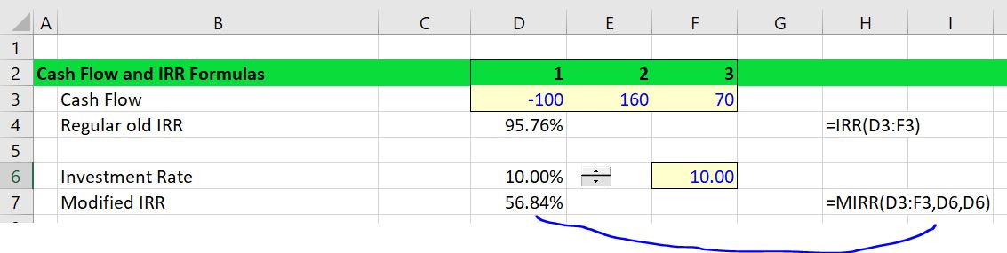
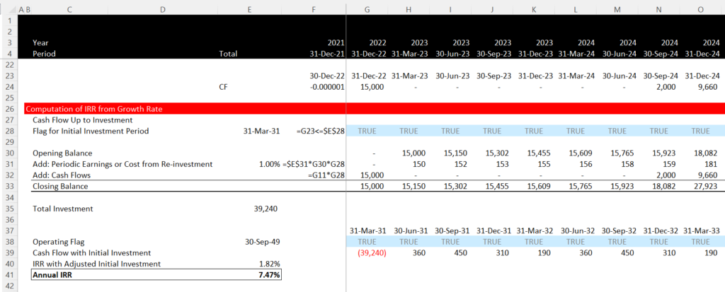
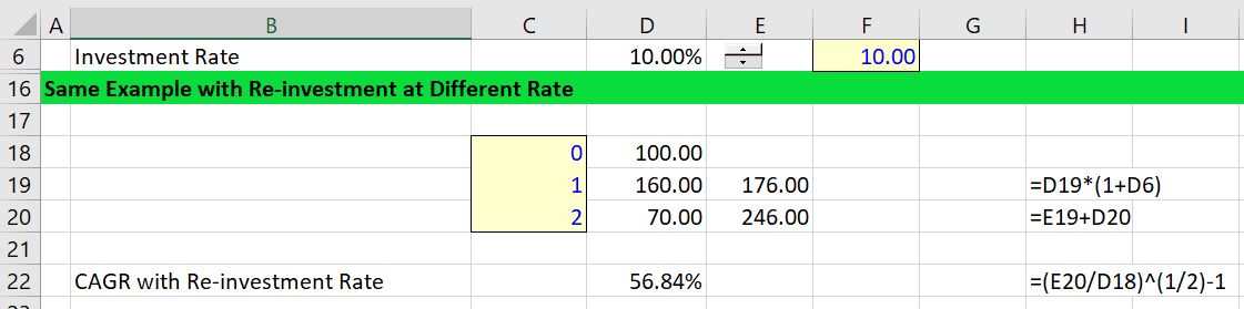
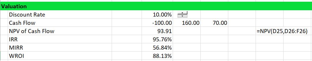
Now lets move to the case with middle year cash flows. I have constructed a very extreme example to demonstrate problems with the re-investment rate. In this example I assume that the second period cash flow is 160 and the third year cash flow is 70. These cash flows produce a very high IRR of 95.76%. Something called the modified IRR (MIRR) can also be computed when you have cash flows between the investment period and the terminal period. If a 10% discount rate is applied, the MIRR is much less than the regular IRR. In the example below, the MIRR is 56.84% as demonstrated in the screenshot. (You can watch to video below to see how these statistics are computed and how to colour the sheet). The screenshot demonstrates how to compute the MIRR using the MIRR formula where you have to enter a discount rate. This MIRR calculation is shown in the next screenshot.
.
.
Multiple IRR’s with Positive, Negative, Positive Cash Flows (EBL Problem)
.
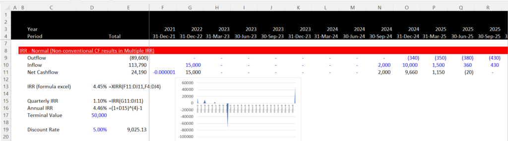
There are situations where there is no discount rate that makes the NPV equal to zero. To address these questions you can go back to the definition of the IRR as a cash account or a positive cash account followed by a negative cash account. I use an example that was given to me by somebody in one of my very favourite companies. The cash flow is illustrated below in the screenshot. When the terminal value is 50,000 you get an IRR computed.
.
.
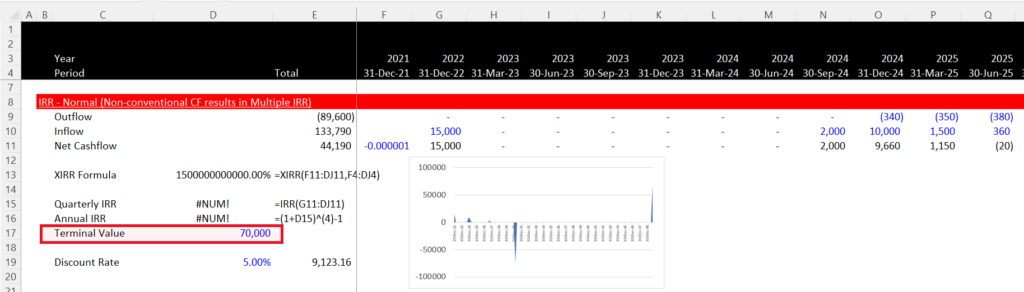
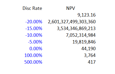
In this example, you can see that the XIRR gives the same answer as the IRR. If the terminal value is increased to 60,000 then the XIRR no longer works. If the terminal value is increased to 70,000, the IRR cannot be computed as shown in the screenshot below. The XIRR gives and absurd answer and the XIRR for some reason gives the initial cash flow. The second screenshot shows that with a terminal value of 70,000 there is no value that gives you an NPV of zero. In this case it is understandable if you say that the IRR seems to make no sense. The spreadsheet with the numbers are available for download below.
.
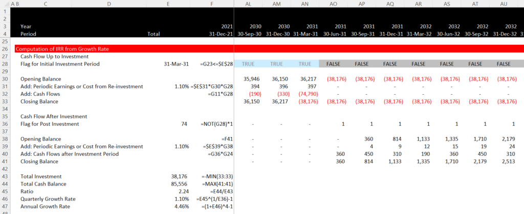
You can compute positive and negative cash flow balance and then compute the growth rate. When you do this, you can computed the accumulated investment using the IRR itself as both the finance rate and the re-investment rate. As with the case above this exercise demonstrates that the IRR is essentially a growth rate. Quarterly cash flows are used in the example and the example splits the cash flows in the big investment period. The example also uses the terminal value of 50,000 so that the IRR can be computed.
.
Next, we can move to the case where the terminal value is 70,000 and the normal IRR cannot be computed. One way to compute the IRR is to put a given borrowing rate into the cash flows before the big cash outflow period. Once the investment is measured in this way, you can then compute the net investment at the date the large cash outflow occurs. You can do this using the same method as illustrated above where a cash account is accumulated, but the income on the cash is not computed using the IRR itself because you do not have the IRR.
.
.
MIRR is B.S. and Does Not Mean Much
Somebody who copied my XMIRR function even stated:”Despite the arguable superiority of the Modified Investment Rate of Return (MIRR) in analyzing investments or capital budgeting decisions …” I will show that this idea that the MIRR is superior to IRR is complete and utter B.S. (Note that you can find documentation of how to create a UDF function on this website.) You should already be asking, what in the heck is going on with the MIRR. If I took my money out of in year 1 and then threw away the last pot of money, my IRR would be 60%. The other 70 in the third period is just an extra amount without any investment. You should already be saying the MIRR is crap.
To illustrate how the IRR and the MIRR produce growth rates in money, I have made a couple of screenshots. In the first screenshot, the IRR is verified. This is done by taking the second period cash flow and then increasing it by a growth rate of 95.76%. (This is the problem with circularity in the IRR calculation and why you may need a guess — you need the IRR to compute the IRR). When you multiply the second period cash flow of 160 by (1+IRR or 1+95.76%) you get a value of 313.21. This is the value of the 160 that grows to the third year. The 313.21 is added to the 70 of cash flow that you get directly to produce a total number of 383.21. Finally, you can divide the 383.21 by 100 and raise the result to the one half power and subtract 1 to compute the compound growth rate (383.21/100) ^ (1/2) – 1 or 95.76%.
.
The MIRR can be demonstrated by the same process in the screenshot below. In this case second year cash flow of 160 grows by the assumed re-investment rate of 10% rather than the IRR itself. (There is no circular reference now). This time the 160 grows to 176 instead of 313.21. When the 176 is added to the last year cash flow of 70, the total last year cash flow is 246. When the compound growth rate is computed from the 246 (246/100)^(1/2)-1, then the growth rate of 56.84% is the same is the MIRR shown in the above example.
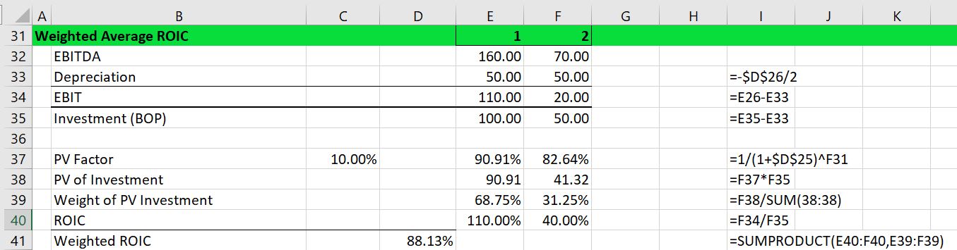
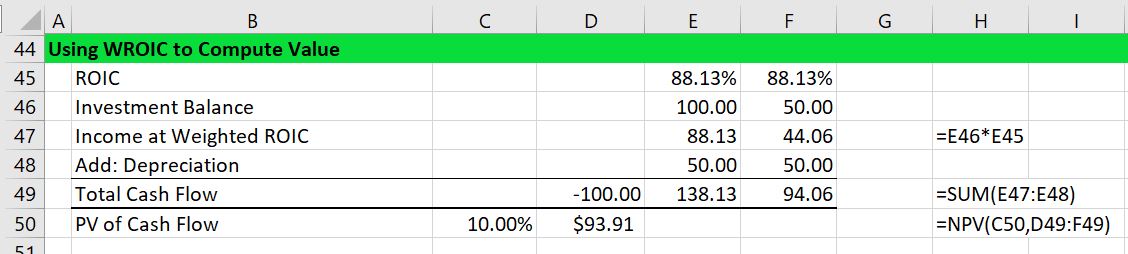
The screenshot below demonstrates calculation of the Weighted Average ROI. First, the ROI is computed from the cash flow. The only calculation required is for depreciation expense. In this simple case the 100 is just divided by 2 for a depreciation value of 50. The cash flow or EBITDA of 160 and 70 is less the depreciation of 50 produces the EBIT. Note that you could include the taxes to use NOPAT or you could use the earnings after tax. In addition, you can compute the nominal value of the investment as the starting investment of 100 less the accumulated depreciation. The beginning of period investment is 100 for the first year and 50 for the second year.
Now, if you were earning a return of 15% per year for two years, but the investment balance was half as much in the second year compared to the first year, the return of 15% should be given less weight for the second year. To extend the example, if you were earning 10% in the first year and 20% in the second year, you could not say that the average return was 15%. This is because the basis for the investment is much less for the second year than for the first year. To resolve this you could weight the investment value.
You are not finished however. If you are comparing money across time, you should always discount the money that occurs in later years. In the example above with 10% and 20%, you should not only account for the lower nominal value of the investment, but you should discount the value of the investment. This would further weight the average towards 10% and away from 20%. In the screenshot below, the investment value is discounted at a rate of 10%. The ROI for the first year is 110% and the return on investment for the second period is 40%. When weighting these return by the present value of the investment the overall weighted average return statistic is 88.13% as shown below. I will argue that this statistic is a better representation of the true value of the investment if the discount rate is 10% than either the MIRR or the IRR.
.
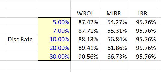
To illustrate the effect of the weighted average ROI versus the MIRR and the IRR with different discount rates, you can look at the data table in the screenshot below which applies different discount rates in the MIRR and WROI calculations. In this case shown below, both the MIRR and the weighted ROI (WROI) increase with the discount rate. This is because the second period return is below the first period return. The data table shows that the weighted average ROI does not produce the illogical result that results from the MIRR where the rate of return is less than 60% (recall that you could take your money after year 1 and earn 60%). The IRR of 95.76% does not change with the discount rate.
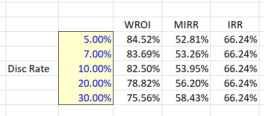
If the cash flows are switched around with the 160 coming at the end and the 70 coming in the middle, the relationship between the IRR and the MIRR changes. In this case the more typical increase in ROI over time occurs (with growth in cash flow and declines in investment). In the table, the MIRR increases with the re-investment as usual as shown in the screenshot below. But this time, since the ROI increases over time, the higher the discount rate, the lower the weighted average ROI. This decline in return as risk increases makes sense as the discount rate or the re-investment rate is supposed to increase with higher risk. With higher risk, value is reduced and the weighted ROI that gives and indication of value is reduced.
You may say that the discount rate applied in the WROI and the MIRR may not necessarily be the cost of capital. But use of the cost of capital for the re-investment rate is discussed by McKinsey: “Most practitioners would agree that a company’s cost of capital—by definition, the return available elsewhere to its shareholders on a similarly risky investment—is a clearer and more logical rate to assume for re-investments of interim project cash flows.” It is easy to understand that MIRR increases with a higher re-investment rate. But it is not easy to understand that a number that is supposed to represent value decreases as risk declines.
Valuation and Weighted ROI
The weighted ROI that I demonstrated above has advantages relative to the MIRR or the unadjusted IRR as a measure value. To demonstrate this, income is calculated as the weighted ROI multiplied by the nominal investment value over the investment period. The income from this calculation is added to depreciation resulting resulting in cash flow that would result from a constant ROI. If the cash flow from this constant ROI is discounted at the same rate as used in the weighted average ROI calculation, the valuation result is the same as the standard NPV calculation. This means if you would rank different investments using the weighted ROIC, the ranking would be the same as the ranking from the NPV technique.
The process of computing income from the weighted average ROI is illustrated in the two screenshots below. In the first screenshot the value of the cash flow is demonstrated. Using a 10% discount rate, the net present value is 93.91.
.
The second screenshot demonstrates calculation of the net present value using weighted average ROI. The weighted average ROI of 88.13% is multiplied by the investment balance to compute hypothetical income. The income is 88.13 in the first year (88.13% x 1000) and 44.07 in the second year (88.13% x 500). This income is added to depreciation of 50 to arrive at hypothetical cash flow. The cash flow is different from the original cash flow, but when discounted it produces the same value of 93.91 as discounting the original cash flow.
.
.
McKinsey IRR B.S.
In an article written in 2004, McKinsey makes a critique of the IRR in terms of capital investment decisions. The McKinsey makes the point that as the IRR implicitly assumes that intermediate cash flows are re-invested at the IRR itself, it is possible come up with situations where the IRR criteria and the NPV criteria produce different results. You can find these points in the link below:
The McKinsey article authors make a dramatic accusation:
“For decades, finance textbooks and academics have warned that typical IRR calculations build in reinvestment assumptions that make bad projects look better and good ones look great. Yet as recently as 1999, academic research found that three-quarters of CFOs always or almost always use IRR when evaluating capital projects.
Our own research underlined this proclivity to risky behavior. In an informal survey of 30 executives at corporations, hedge funds, and venture capital firms, we found only 6 who were fully aware of IRR’s most critical deficiencies. Our next surprise came when we reanalyzed some two dozen actual investments that one company made on the basis of attractive internal rates of return. If the IRR calculated to justify these investment decisions had been corrected for the measure’s natural flaws, management’s prioritization of its projects, as well as its view of their overall attractiveness, would have changed considerably.”
McKinsey advocates use of NPV rather than IRR and use of the MIRR to fix the famous re-investment problem. In the discussion below I explain the article is largely rubbish. I explain that the MIRR does not fix anything at all and the WROI would be a much better ranking method. I begin with a five year cash flow case used in the McKinsey article.
Ranking of Investments with the Same Life
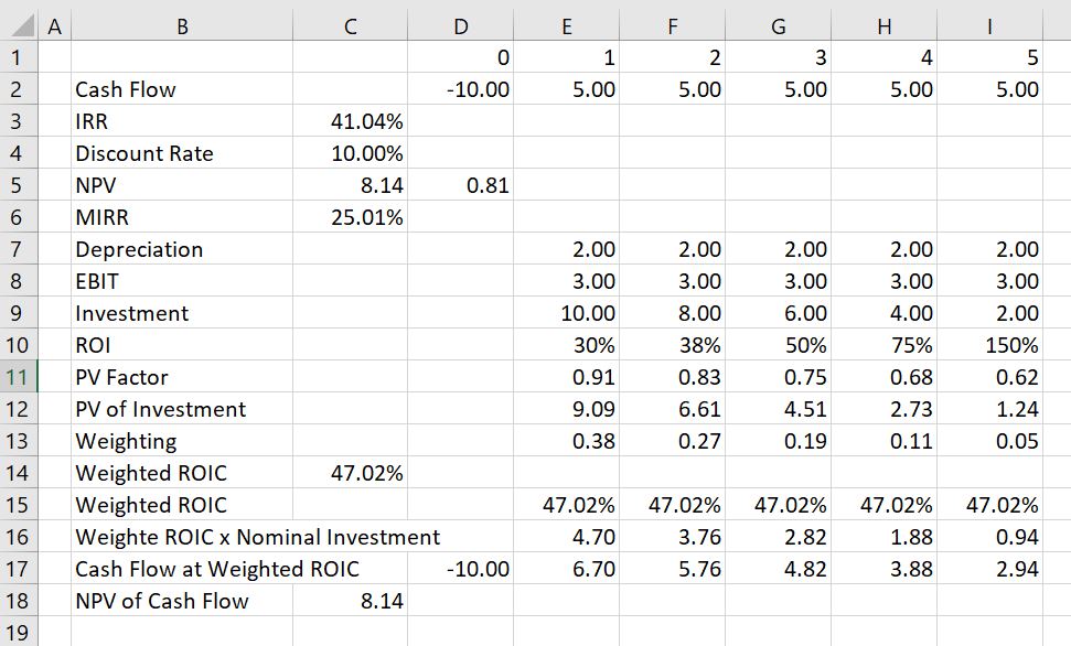
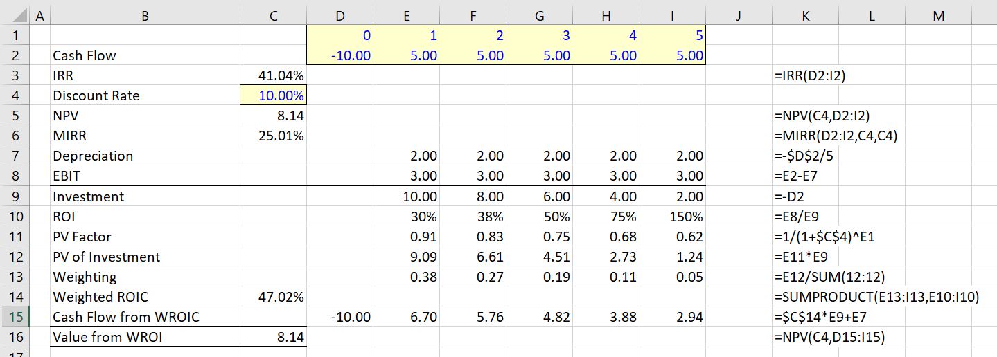
To illustrate how the IRR can distort ranking of investments begin with the example used in the McKinsey article. This case has an outlflow of 10 followed by positive 5 cash flow for 5 years. This cash flow produces an IRR of 41.04%. With a discount rate of 10%, the MIRR is 25.01% and the weighted average ROI is 47.02%. The reconciliation of the NPV of 8.14 is confirmed with the NPV from the weighted ROI in the screenshot below.
Next consider a case where there are no middle year cash flows and the final cash flow in period is 50. The cash flow of 50 is much more than the 5 years of cash flow of 5 that adds up to 25. But because of timing, the unadjusted IRR is lower than the first case. The IRR is 37.97% as shown in the screenshot below. But when the NPV is computed at a discount rate of 10% the NPV of the investment is higher — it is 19.13 rather than 8.14. This is thus a classic case of different ranking for NPV and IRR. The first investment with 5 years and a cash flow of 5 has a better ranking from the IRR than the investment shown in the screenshot below. But the first investment above has a lower ranking than the investment shown below when the NPV is used. The correct decision would be to use NPV and take the second investment.
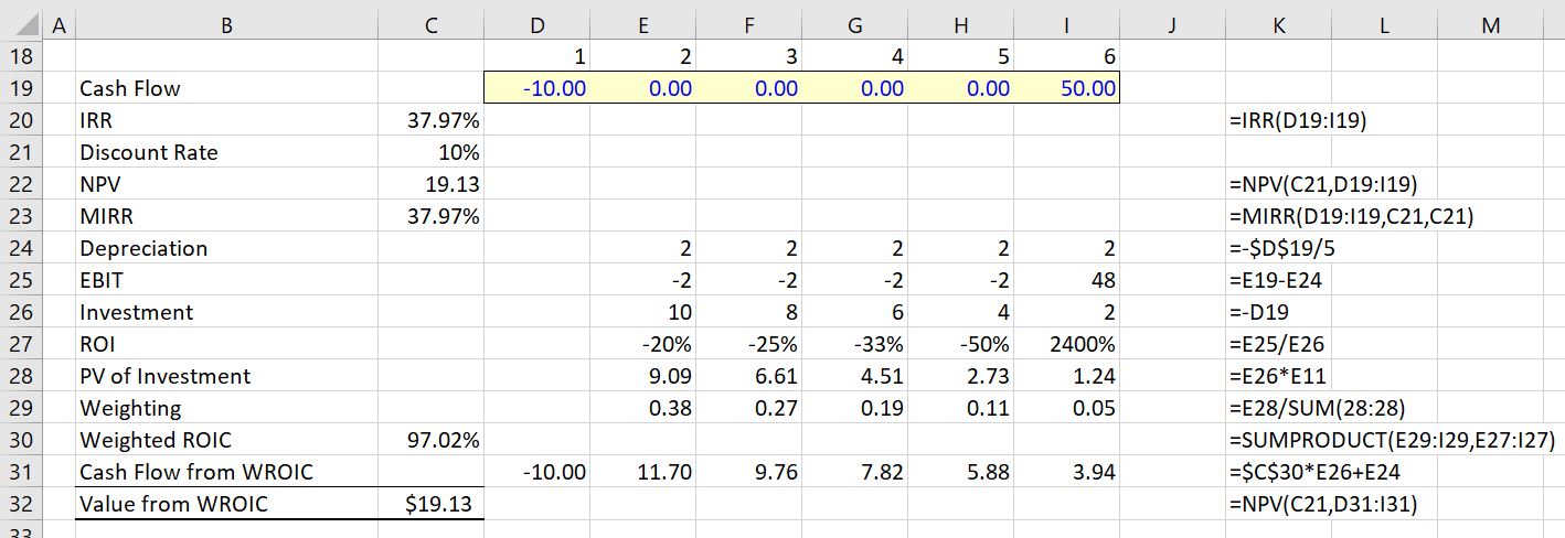
When looking at the above screenshot, you can see that MIRR of 25.01% is lower for investment 1 than for investment 2 where the MIRR is the same as the overall IRR of 37.97%. The MIRR is the same in the second case because there are no middle period cash flows. In the first case, the MIRR is lower than the IRR because the middle cash flow earns a lower return than the overall IRR. In terms of the WROI, the ranking is the same as the correct ranking where the second investment has a very high WROI. The MIRR of 25.01% for the first investment is lower than any of the ROI.
When the calculated IRR is higher than the true reinvestment rate for interim cash flows, the measure will overestimate—sometimes very significantly—the annual equivalent return from the project. The formula assumes that the company has additional projects, with equally attractive prospects, in which to invest the interim cash flows. In this case, the calculation implicitly takes credit for these additional projects. Calculations of net present value (NPV), by contrast, generally assume only that a company can earn its cost of capital on interim cash flows, leaving any future incremental project value with those future projects.
The McKinsey article discusses the problem with the following jiberish: “IRR’s assumptions about reinvestment can lead to major capital budget distortions. Consider a hypothetical assessment of two different, mutually exclusive projects, A and B, with identical cash flows, risk levels, and durations—as well as identical IRR values of 41 percent. Using IRR as the decision yardstick, an executive would feel confidence in being indifferent toward choosing between the two projects. However, it would be a mistake to select either project without examining the relevant reinvestment rate for interim cash flows. Suppose that Project B’s interim cash flows could be redeployed only at a typical 8 percent cost of capital, while Project A’s cash flows could be invested in an attractive follow-on project expected to generate a 41 percent annual return. In that case, Project A is unambiguously preferable.”
“Even if the interim cash flows really could be reinvested at the IRR, very few practitioners would argue that the value of future investments should be commingled with the value of the project being evaluated. Most practitioners would agree that a company’s cost of capital—by definition, the return available elsewhere to its shareholders on a similarly risky investment—is a clearer and more logical rate to assume for re-investments of interim project cash flows (Exhibit 1).”
Case with Projects that have Different Lives Demonstrating Problems with MIRR
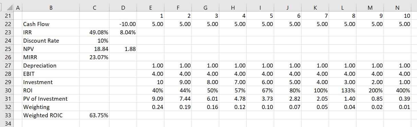
When investments with different lives are ranked, the MIRR falls apart as a statistic. On the other hand, the weighted average ROI continues to correctly value different projects. To illustrate this, compare the case with 5 years of 5 cash flow to a case with 10 years of 5 cash flow. If the investment is the same, it is pretty obvious that you would rather have the longer cash flow. But the MIRR gives a lower return to the longer cash flow because it compresses cash flows to the re-investment rate. The longer term cash flow project would be ranked lower than the project with shorter cash flow.
To illustrate this case, return first to the 5-year case. This is a repeat of the screenshot above with an IRR of 41.04% with an MIRR of 25.01% and a weighted ROIC of 47.02%. The NPV of the investment is 8.14.
In the second case where the cash flows are simply extended, the IRR increases to 49.08% (not too much) and the MIRR declines from 25.01% to 23.07%. The NPV of the investment more than doubles from 8.14 to 18.84. Thus, the MIRR would actually suggest that the investment below is worse than the investment with only 5 years of cash flow. The MIRR is not consistent with the NPV. The NPV is B.S.
On the other hand, the WROI increases dramatically as did the NPV. It increases from 47.04% to 63.75%.
Videos that Describe WROI as an Alternative to MIRR or IRR
The three videos below describe the problems with IRR when you have middle period cash flow. It is demonstrated that a weighted average return solves problems with the IRR in terms of measuring growth and ranking investments.
[wonderplugin_video iframe=”https://www.youtube.com/watch?v=mjlNTAP8rbo&t=120s” videowidth=600 videoheight=400 keepaspectratio=1 videocss=”position:relative;display:block;background-color:#000;overflow:hidden;max-width:100%;margin:0 auto;” playbutton=”https://edbodmer.com/wp-content/plugins/wonderplugin-video-embed/engine/playvideo-64-64-0.png”]
[wonderplugin_video iframe=”https://www.youtube.com/watch?v=4Npyc2K40Vk&t=5s” videowidth=600 videoheight=400 keepaspectratio=1 videocss=”position:relative;display:block;background-color:#000;overflow:hidden;max-width:100%;margin:0 auto;” playbutton=”https://edbodmer.com/wp-content/plugins/wonderplugin-video-embed/engine/playvideo-64-64-0.png”]
[wonderplugin_video iframe=”https://www.youtube.com/watch?v=YwwNgFuhgn0&t=26s” videowidth=600 videoheight=400 keepaspectratio=1 videocss=”position:relative;display:block;background-color:#000;overflow:hidden;max-width:100%;margin:0 auto;” playbutton=”https://edbodmer.com/wp-content/plugins/wonderplugin-video-embed/engine/playvideo-64-64-0.png”]
Comments on IRR
I purchased your book several years ago and just stumbled on your website/youtube videos the other day. Your latest videos on IRR/MIRR caught my attention as I’ve had the same arguments regarding IRR several times, and your WROIC is interesting. I messed around with the excel document and it seems to improve on some shortcomings of IRR and NPV. It does a better job capturing investment life (with equal NPVs, equal investment, a shorter investment life gives a higher WROIC), and investment amount (with equal NPVs, equal life, a lower investment yields a higher WROIC), and having that captured in a single metric is very useful for a management team that wouldn’t usually be familiar with the details of various projects/investments under consideration.
Getting management teams on board always seems to be the greatest challenge, and one thing I see causing confusion is the Depreciation, as in this calculation it doesn’t necessarily tie to either Tax or Book depreciation, but just the project/investment life. I haven’t tried the WROIC calculation in a full model with multiple investment periods, but while the NPV of Cashflow at Weighted ROIC is fine when you just add another period of negative cash flow, the Weighted ROIC is incorrect. Starting the calculation following the last investment period seems to solve the problem, is that how you recommend doing it?
That McKinsey article is utter garbage, but unfortunately has been cited numerous times. IRR certainly has problems, but whoever wrote the advice the article provides is beyond terrible. Like I mentioned I’ve had the “IRR is only accurate when proceeds can be reinvested at the same rate” argument several times and the best way I’ve seen to that isn’t correct is the example below. Create a simple project model and solve for the IRR, then create a bank account earning interest at the IRR of the project, where negative cashflows are deposits and positive cashflows are withdrawals. It’s clear here that your account balance is earning the IRR, and the cashflows taken out doesn’t need to be reinvested anywhere.
| Project/Investment | |||
| Period | 0 | 1 | 2 |
| Investment | (100) | ||
| Return | – | 130 | |
| Total Cashflow | (100) | – | 130 |
| IRR | 14.02% | ||
| Bank Account Earning Interest at IRR | |||
| Account Balance | 100.00 | 100.00 | 114.02 |
| Interest Earned | – | 14.02 | 15.98 |
| Account Balance End of Period | 100.00 | 114.02 | 130.00 |
| Withdrawal | – | – | (130) |
| Account Balance After Withdrawal | 100.00 | 114.02 | (0.00) |
| Project/Investment | |||
| Period | 0 | 1 | 2 |
| Investment | (100) | ||
| Return | 160 | 70 | |
| Total Cashflow | (100) | 160 | 70 |
| IRR | 95.76% | ||
| Bank Account Earning Interest at IRR | |||
| Account Balance | 100.00 | 100.00 | 35.76 |
| Interest Earned | – | 95.76 | 34.24 |
| Account Balance End of Period | 100.00 | 195.76 | 70.00 |
| Withdrawal | – | (160) | (70) |
| Account Balance After Withdrawal | 100.00 | 35.76 | (0.00) |
The other thing I’ve shown people is how to replicate the MIRR function by just trapping all the positive cashflow from a project, earning the reinvestment rate on the cumulative balance, and releasing it at the end of project life. That makes it pretty clear that MIRR isn’t really a Modified IRR, but it really modifies the project cashflows and then does the same calculation as a regular IRR.