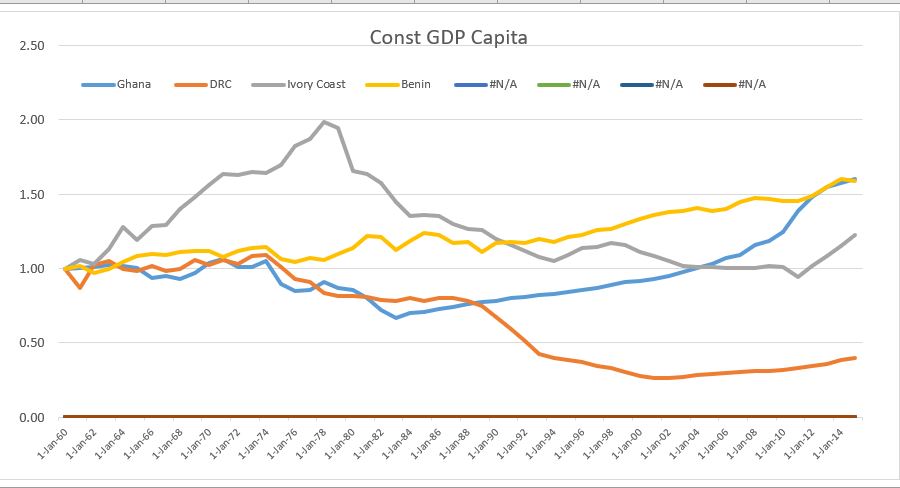
This webpage shows you how to put varying numbers of data series on graphs (e.g. you can add a new stock to a stock price graph). Here, you may want to graph one stock compared to the growth index of GDP or you may want to graph five different stocks against the GDP. To select one, two, three or more series on a graph, the list box form in excel can be used (for example, say you want to graph four stock price items instead of two stocks). Alternatively you can make a series of TRUE/FALSE switches with list boxes. With the list box using the multi-entry option you can one or two or four or ten etc, series on a graph by clicking on the item in the list box. Creating list boxes is not a big deal if you are not using the multi-select option. But implementing the list boxes for making a really flexible graph using the multi-entry option does require a little VBA code that you should not be afraid of. Whether you are using the list box or the TRUE/FALSE switch method, you can develop the process using the MATCH function.
Using a List box Form with Multiple Selections to Allow Different Series to be Presented on a Graph
A thing that I have not been able to do for years is to be able select either a different number of series on a graph with a list box. By this I mean you may for example want to pick two different countries or alternatively ten countries to display on a graph. In looking at the list box from the developer tab, I thought it must be easy to select multiple items from the list box and then create a graph with a flexible number of stock prices, countries, interest rate series, currencies etc. I was wrong about this. I could not find a simple explanation of how to make a list box with multiple entries that could be used to adjust a graph. If you could make a list box with multiple entries, you could then choose to not show one series on a graph by deselecting the item from the list box.
Step 1: Insert the List Box from the Developer Tab
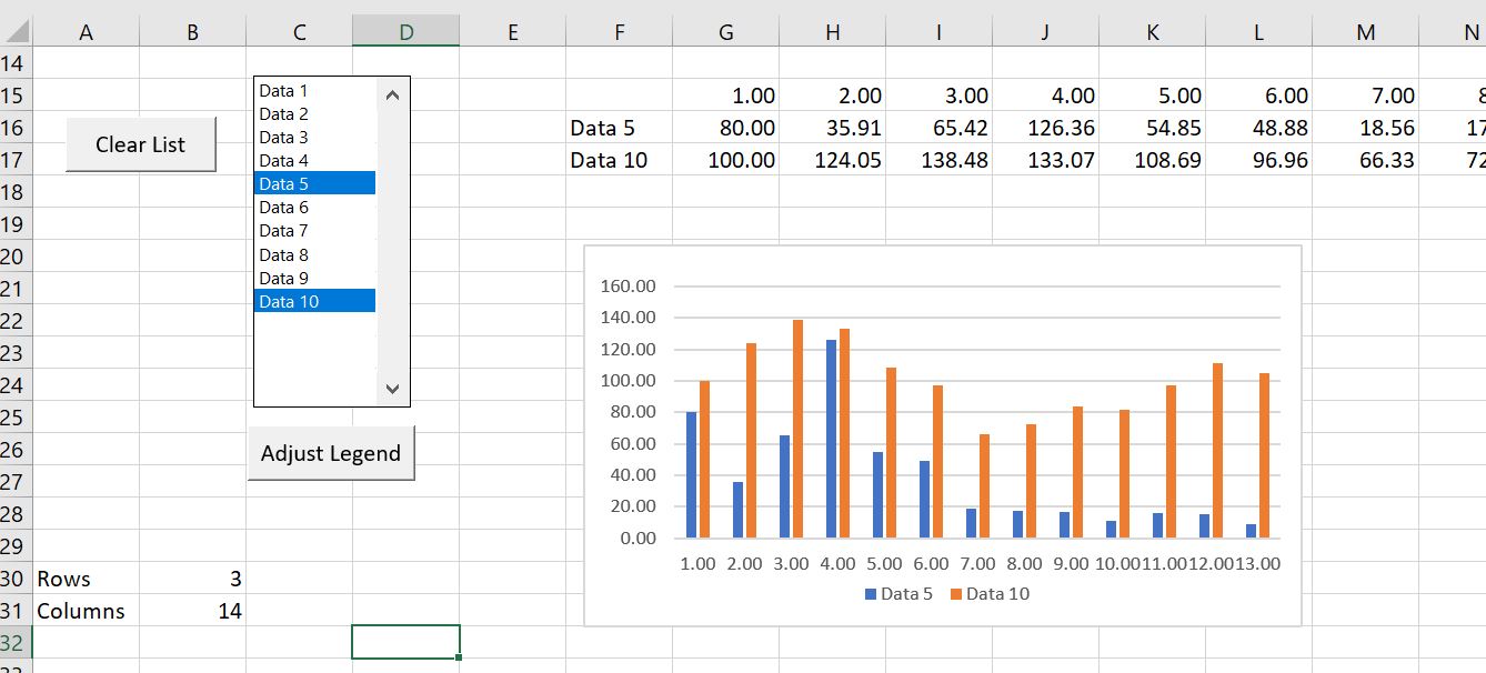
To use a list box in a graph or in other circumstances with multiple entries you need to add a macro to the list box. This process is illustrated in the file below that has macros that allow you to use the LIST BOX Form with MULTIPLE selections. The manner in which a list box can be used to select multiple entries is illustrated in the screenshot below. You can download the associated file that allows to select the different series in a graph is available for download just below the screenshot.
Step 2: Attach VBA Code to List Box that Produces the Name of the Item in the Listbox as the Output
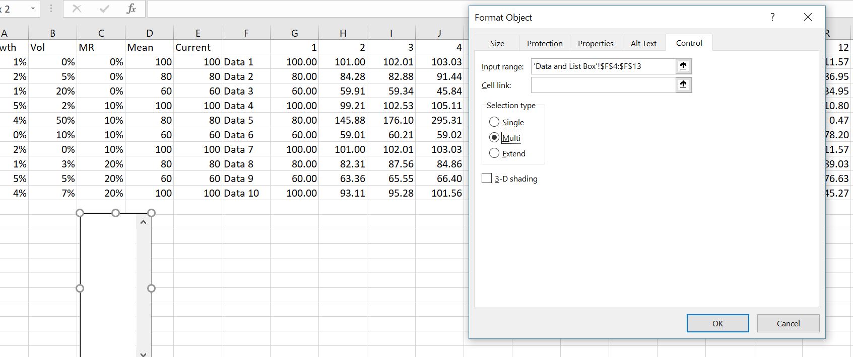
To implement the list box, you need to have the developer tab installed from the customise menu option (or the customise ribbon after you go to the options from the file menu). The screen shot below illustrates how to make a list box and then select the multiple selection option — note that the Multi option is selected. After you right click on the list box form, click on the “Mutli” option and leave the cell link blank.
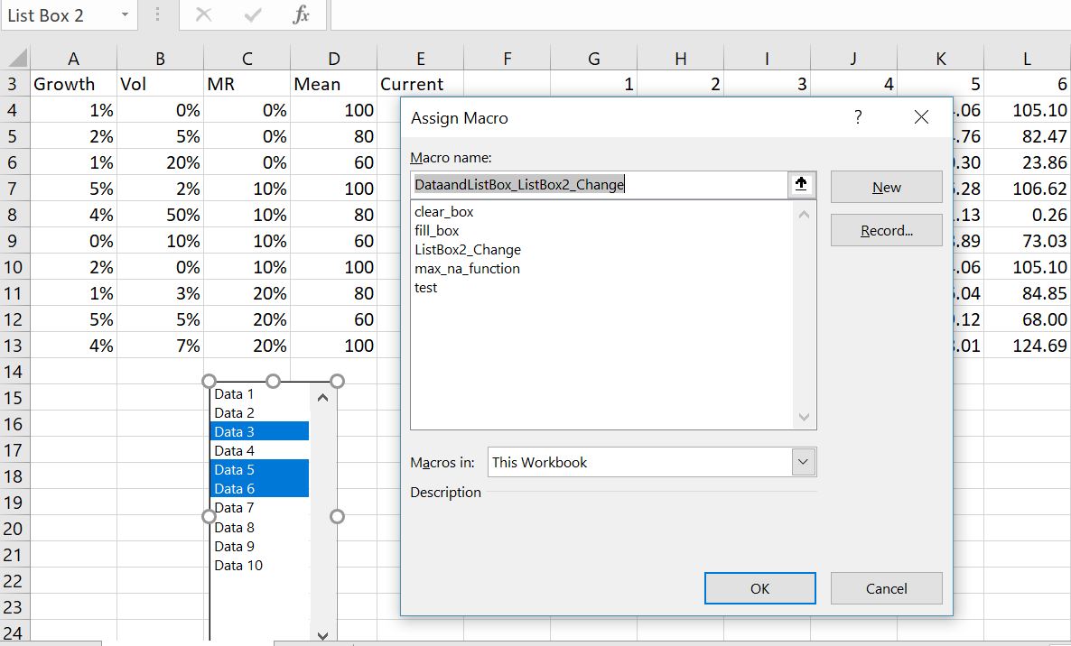
Once you have put a list box in your sheet, you need unfortunately to attach some VBA code to the list box. You need to find the name of the list box (e.g. LIST BOX 2) and then attach a macro to the list box. To find the name of the list box you can attach a macro to it and then the macro code will show the name. Then you should edit the VBA code and put in the correct name (e.g. LIST BOX 2) of the list box in the sample code. A file that contains the VBA code (macros) that you can download is the list box template file and you can copy the code in the section below. This sample file contains the macros that you can attach to the list box and allow the list box to spit out the items that have been selected to the spreadsheet. The screenshot below illustrates how to attach the VBA code to the list box. The macro puts the output of the listbox in a range name that is defined used in the VBA code. In the example below, the range name is “listbox_range”.
File with Example of Listbox and Associated VBA Code
To download the file that contains the VBA code is included in the template file that you can download by pressing the button below. To attach the VBA code for the listbox to your file, first press the ALT, F8 key sequence in the listbox template file and press one of the macros. Then after the VBA code is shown, press CNTL, A to collect all of the code and after that press CNTL, C as usual. Then, open your file and press ALT, F8 again (it works best if you select “This workbook” as shown in the screenshot above). Next, type in a macro name like STORMY and click on the edit option. Finally, copy the code to your file by pressing CNTL, V.
Spreadsheet with Listbox Example that Includes VBA Code for Creating Flexible Graphs
Step 3: Creating a Graph from List Box Outputs with MATCH and INDEX of LOOKUP Functions
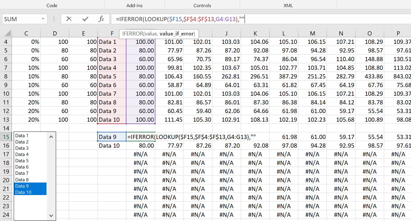
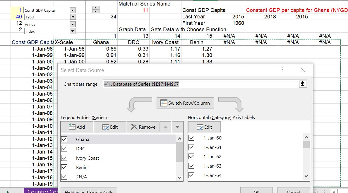
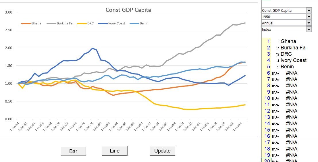
The screenshot below illustrates how you can create a graph from the outputs of the list box. The The list box outputs are in column F and starting in row 15. Once you have these, you can use the MATCH and INDEX functions, the LOOKUP function, or you can create your own function. The names that are selected from the listbox are put in the range listbox_range using the macro code below. Once you have these names, you can use the MATCH function to find the row or column numbers of the bigger list. If the list is in a sorted order, you can use the LOOKUP function as illustrated below.
Repairing Legend to Graphs and Removing #N/A’s
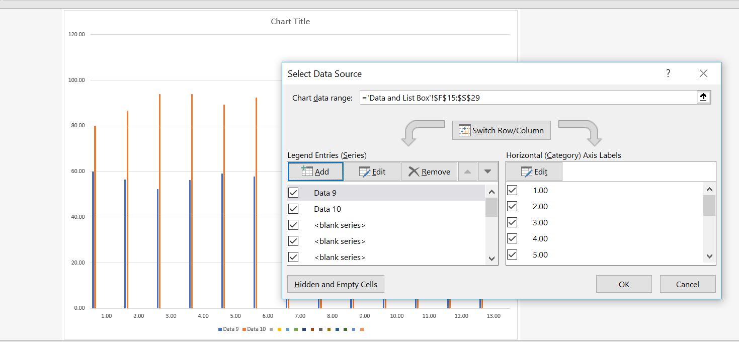
When you create a graph with the listbox per the discussion above, the graph will have #N/A’s for potential series that are not selected. This has been an irritation for me for years. It is tricky to put a legend without #NA in the graphs after you have made the flexible graphs, but it can be done. The screenshot below illustrates the problem where series that are not graphed have the #N/A.
The reason the #N/A’s appear is that the area of the graph must be large enough to capture the maximum amount of series that you would like to appear on the graph. The graph area that is larger than the amount of actual series that are graphed is illustrated on the screenshot below.
Fixing the Problem Step 1: Create Flexible Range Name with Offset
To fix the problem, one way is to make the area more flexible. I thought you could use the OFFSET function with a dynamic range name and then put this into the chart data range as illustrated in the screenshot below. This does not work. When you make the dynamic range with the OFFSET function (by putting in the number of rows and columns in the height and width option), the range name does not stay in the graph.
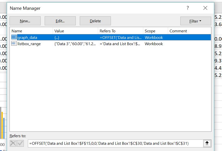
To fix the problem, you still have to make a flexible range name. The number of series to graph and the length of the graph should be defined somewhere. These are the parameters for the height and width of the dynamic range as illustrated below. The start row and the start column should generally be zero. A dynamic range name created with the OFFSET function is illustrated below. Note that the number of rows and the number of columns must include space for the x-axis and the y-axis.
Fixing the Problem Step 2: Create VBA Code to Define Graph Range
You may think all you have to do is to put the flexible range name in the data range part of the graph. This unfortunately does not work as the range name is not maintained. The screen shot below was taken after I put a range name called graph_data into the chart data range. After clicking again on the chart, the range name goes away.
To make the range name stay in the graph, or more precisely, change the graph when the listbox changes, you can make a little VBA code. You need to first activate the chart name. You can find the chart name by right clicking on the chart name and then going to assign macro. You do not have to assign a macro, just do this to find the chart name. In the screenshot below, the chart name is chart1.
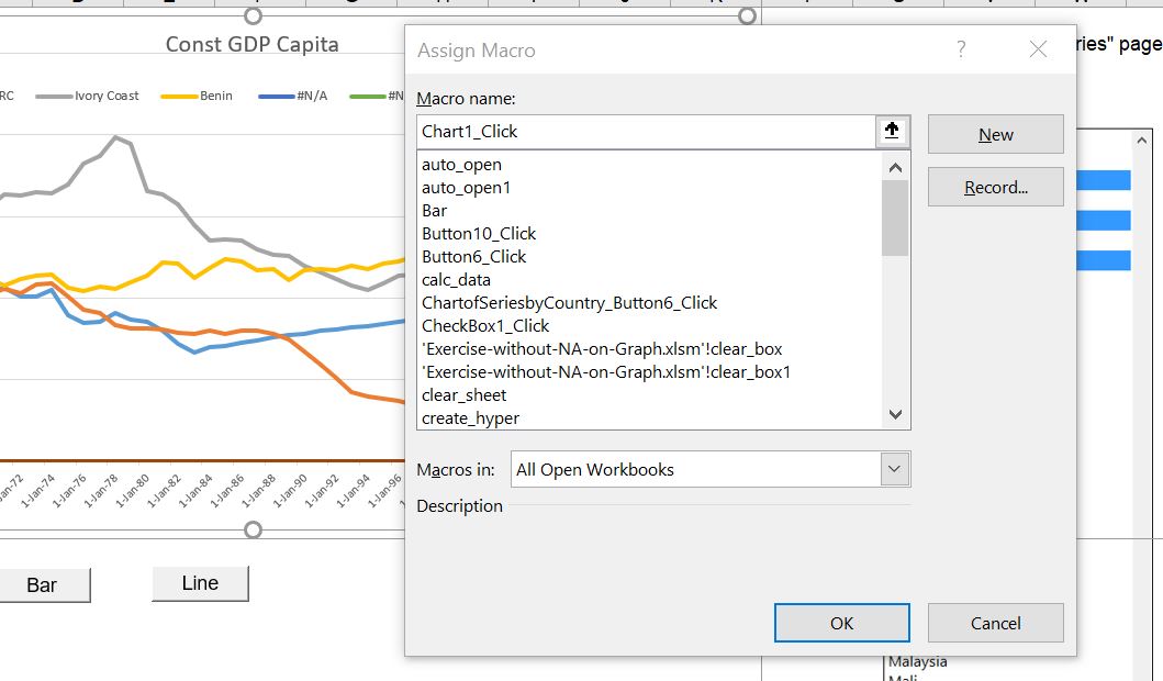
After you find the chart name, copy the VBA code below into your file. You can press the ALT, F8 key sequence and then edit any macro. Just copy the macro and modify the chart name and, if necessary, the range name.
Finally, create a button with something like “update chart” as the name. Then assign the macro you just copied to that range name. The final chart should look something like below. Now, when you change the number of series on the graph, you should hit the update button. (Note, you may have to work with the x-scale a bit).
File that Includes Example of Adjusting the #N/A Legend Problem
A file that includes the VBA code to create flexible charts with legends that change is available for download by clicking on the button below. In this file you can press the CNTL and F3 sequence to see the dynamic range name. This range name (graph_data) changes when the list box changes and different numbers of graphs are selected. When you click the box named “adjust legend”, the legend should change.
The VBA code that allows you to remove the blanks or the #NA’s from the legend is shown below. You can either code into the macro for the listbox or you can include a separate macro.
Sub Adjust_legend()
'
'
 current_cell = ActiveCell.Address

 ActiveSheet.ChartObjects("Chart 8").Activate

ActiveChart.SetSourceData Source:=Range("graph_data")

 Range(current_cell).Activate

End Sub
Video Explanations of Listbox
Lets say you are not interested in macros but you want to use this listbox process you can just copy it from the listbox in the file to a listbox in your workbook. If you download the file, you can right click on the list box, select the macro and copy it to your file. You just have re-name the list box number in the macro. The list box can be effective in making graphs where you may want to present a different amount of series. For example, you may want to compare 10 stocks or only two stocks on a graph. The problem is that to use the LISTBOX you need to attach it to a macro to collect data from multiple sources. This macro and process is demonstrated in the file.
[wonderplugin_video iframe=”https://www.youtube.com/watch?v=X66q4aRZaFM” videowidth=600 videoheight=400 keepaspectratio=1 videocss=”position:relative;display:block;background-color:#000;overflow:hidden;max-width:100%;margin:0 auto;” playbutton=”http://edbodmer.com/wp-content/plugins/wonderplugin-video-embed/engine/playvideo-64-64-0.png”]
.
[wonderplugin_video iframe=”https://www.youtube.com/watch?v=N2M_1mTHjtQ” videowidth=600 videoheight=400 keepaspectratio=1 videocss=”position:relative;display:block;background-color:#000;overflow:hidden;max-width:100%;margin:0 auto;” playbutton=”http://edbodmer.com/wp-content/plugins/wonderplugin-video-embed/engine/playvideo-64-64-0.png”]
.
[wonderplugin_video iframe=”https://www.youtube.com/watch?v=M88W5382QD8″ videowidth=600 videoheight=400 keepaspectratio=1 videocss=”position:relative;display:block;background-color:#000;overflow:hidden;max-width:100%;margin:0 auto;” playbutton=”http://edbodmer.com/wp-content/plugins/wonderplugin-video-embed/engine/playvideo-64-64-0.png”]
.
[wonderplugin_video iframe=”https://www.youtube.com/watch?v=eLCEcY1bWSc” videowidth=600 videoheight=400 keepaspectratio=1 videocss=”position:relative;display:block;background-color:#000;overflow:hidden;max-width:100%;margin:0 auto;” playbutton=”http://edbodmer.com/wp-content/plugins/wonderplugin-video-embed/engine/playvideo-64-64-0.png”]
.
Excel File with Demonstration of How to Create Listboxes that Is Described in the Associated Video
Excel File that Illustrates the Use of Named Ranges in Creating Listbox with Multiple Entries
Link to My Youtube Channel Where You Can Look At All of the Different Videos that I have Made
VBA Code for Listbox
The VBA code that allows you to output the selected list is shown below.
Sub ListBox3_Change()

start_cell = ActiveCell.Address ' takes you back out of the list box

total_rows = Range("listbox_range").Rows.Count ' find the total rows in the listbox

For i = 1 To total_rows
 Range("listbox_range").Cells(i, 1).Clear ' clear out the range name that will be re-filled
Next i

ActiveSheet.Shapes.Range(Array("List Box 2")).Select ' IMPORTANT change this name to the number of your box

Row = 1 ' Make a row counter to put output

For i = 1 To Selection.ListCount ' This is the number in the list box
 If Selection.Selected(i) = True Then ' Only keep the selected items

 Range("listbox_range").Cells(Row, 1) = Selection.List(i)

 Row = Row + 1 ' Assign to the range name
 End If
Next i ' Finish loop around the listbox items

Range(start_cell).Select

End Sub