This page addresses how you can make adjustments for debt financing in a levelised cost analysis which means accounting for the cost of debt in the analysis and using a target equity IRR to compute the levelised cost. I present two alternative methods with associated proofs. The first applies project finance principles where you input things like the DSCR on the P90 and the tenor of the debt. The second, which is more theoretically correct in my opinion applies corporate finance principles with a constant capital structure. This can be thought of as continuing re-financing in a project finance context. When you use the second corporate finance or continuing re-financing method, you can can compute the WACC with the pre-tax and the after-tax interest rate. Using the WACC method, the trickiest and most useful part is demonstrating how to reconcile the method with project financing. I have reconciled the WACC and the project financing using economic depreciation to compute the capital over time and the debt capital over time. This can be used to compute the implicit debt repayment by period to maintain an economic capital structure.
Proving the Carrying Charge Mechanics with a Financial Model
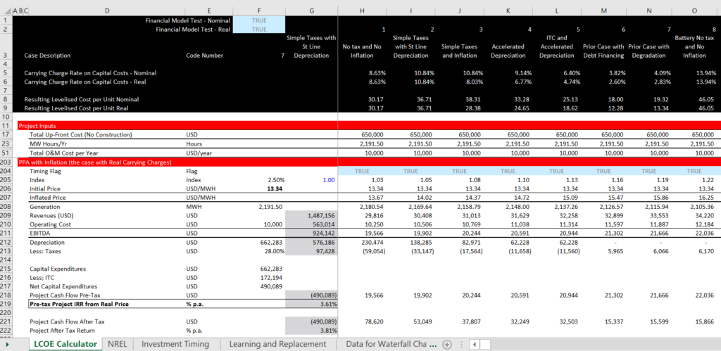
In this section I work through a financial model and demonstrate the LCOE and the results of a financial model are the same thing, just presented in a different way. The LCOE starts with the required IRR and financing assumptions and derives prices. A financial model on the other hand starts with price and derives the IRR. When I received an email blasting me for being so worried about LCOE and carrying charges as being too simple to worry about, the person who sent me the delightful and critical email may have been correct. But I have noticed a whole lot of confusion about LCOE in my work and I am convinced that the economic cost of an asset is essential for very many policy and investment analysis. So I have have created a proof of the LCOE with a financial model as part of the LCOE calculator.
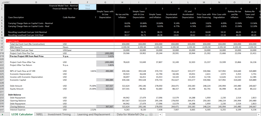
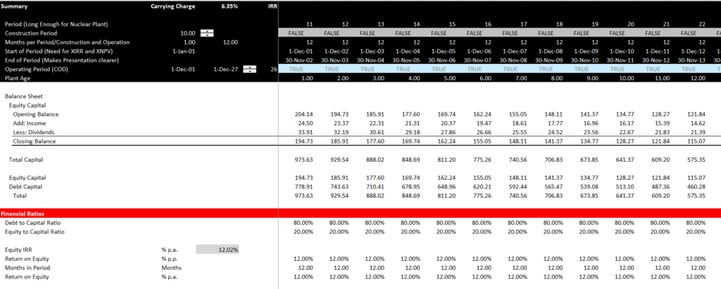
After establishing the pre-tax and post-tax project IRR, you are ready to work on the financing part of a model. The big issue in modelling is often deriving the method of debt repayment. In this example, I use the economic depreciation to compute the capital associated with the project. This economic capital is used to divide the capital between debt and equity. Once you have the debt balance, you can derive the debt repayment. Then, in any model there should always be a debt balance and an interest computation. Note in this case that the after-tax interest rate is below the after-tax project IRR.
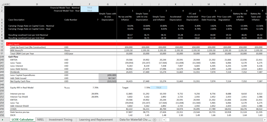
The final part of the model includes a cash flow waterfall and calculation of equity cash flow that includes the initial sources and uses of cash. You can then also derive the DSCR implied by the debt to capital ratio. This last part of the financial model is illustrated in the screenshot below. Note that the target IRR equals the computed IRR and there is a test to confirm the model.
The file that is discussed in this section and the file that includes the equations is attached to the button below.
Excel File with Levelised Cost of Electricity Mechanics Including Detailed U.S. Tax Aspects and ITC
Carrying Charges and Economic Depreciation for Evaluating Capital Structure with Equal Proportions over Project Life
A big difficulty in computing carrying charges with debt and and equity is keeping the capital structure constant. Debt sculpting, mortgage payments or other forms of project finance debt do not keep the capital structure constant. Instead, for computing the debt repayments and keeping the capital structure the same, you can first compute the total capital — just from the capital expenditures. After you compute the total capital associated with the project you can allocate it to debt and equity.
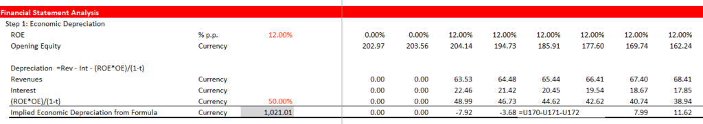
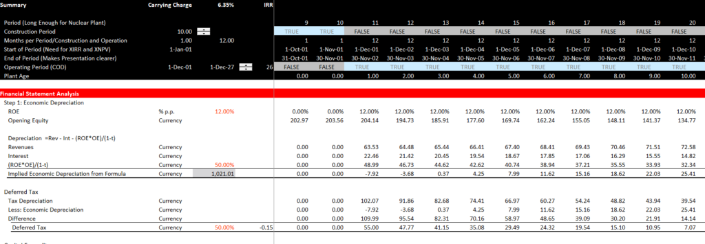
To compute the total capital, the capital must be based on the cash flows. To do this, I insist that you compute the economic depreciation. This is illustrated in the screenshot below. The depreciation is backed out. Start by considering a normal simple income statement:
With economic depreciation, the return is the same when computing the return on the opening balance of the equity. So the income in an income statement is the ROE x the opening equity balance.
With taxes, things get a little more complicated. To compute the economic depreciation with taxes, this income you compute from the opening balance x the ROE can be divided by one minus the tax rate.
Note that this all assumes you can compute the EBITDA from the PMT formula.
- Revenues Less Operating Expense
- EBITDA
- Less Interest
- Less Taxes
- Less Depreciation
- Equals Income
With no taxes and no debt, the Economic depreciation is:
EBITDA – Economic Depreciation = Opening Balance of Capital x Return
EBITDA = Opening Balance x Return + Economic Depreciation
Economic Depreciation = EBITDA – Return * Opening Balance of Capital
With taxes and interest the economic depreciation is:
Economic Depreciation = EBITDA – Interest – After-tax Income/(1-Tax Rate)
Economic Depreciation = EBITDA – Interest – ROE * Opening Balance/(1-Tax Rate)
Videos associated with Levelised Cost
There are a series of videos that describe the various issues associated with computing levelised cost. I am sure there is one correct method to compute the levelised cost that you can prove with a project finance model that includes re-financing and terminal value. I have no idea how you could watch all of these videos without going crazy. But you may want to tak a look at a couple of them.
If you want the filse associated with levelised cost I have the files in a folder (chapter 5, conventional energy) of the resources. Just drop and email to edwardbodmer.com and I will send a google drive with a whole lot of stuff (probably too much). But you can unzip the files and look for what you want and save the google drive in the cloud….
| Carrying Charge Introduction | https://www.youtube.com/edit?o=U&video_id=z9s06nXh7U4 | |
| Carrying Charges and Inflation | https://www.youtube.com/edit?o=U&video_id=9uh8ZN_SHN4 | |
| Taxes in Carrying Charge Rates | https://www.youtube.com/edit?o=U&video_id=n3MWZvnleWg | |
| Periodic Analysis in Carrying Charges | https://www.youtube.com/edit?o=U&video_id=zp06ubSxiGQ | |
| Completed Carrying Charge Analysis | https://www.youtube.com/edit?o=U&video_id=ho2RnSHOWfk |
Files associated Computing Carrying Charges
There are three files associated with this lesson set. The first file is the completed carrying charge analysis that you can use for economic analyses such as the analysis of batteries, solar and diesel. The second file includes all of the components of the carrying charge beginning with the PMT function and ultimately including effects of inflation, taxes, construction timing, replacement and debt. The third file includes exercises that you can work through in order There are a series of videos that describe each of the adjustments that you can make to derive the carrying charge. The video begins by describing the simple PMT function and moves to inflation, tax, depreciation, construction periods, replacement cost and debt.
This page addresses LCOE — the levelised cost of energy and the associated carrying charge rates. LCOE and carrying charge rates are evaluated with through demonstrating how to find data, how to measure and put together all of the factors that drive the carrying charge, and how to use carrying charge rates in economic analysis. For the electricity industry and other capital intensive industries different investment alternatives that have alternative operating lives, capital costs, variable costs, fixed costs and risks the LCOE can be an effective way effectively summarise different alternatives.
LCOE and FAST
Creating a financial model from the LCOE makes you think about some of the fundamental principles of making a financial model. This is to make a well structured, flexible, accurate and transparent model (the FAST letters). Do not worry about silly rules, just keep these ideas in the back of your head somewhere. Flexibility is illustrated by learning how to make time lines in seconds with a differentiation between the pre-COD and post-COD periods. Accuracy is covered by using TRUE/FALSE switches that assure that the balance sheet balances among others. Structured means that you should first compute the project IRR pre-tax; then add taxes; and put the financing in only after the after-tax project IRR is computed. Finally, transparency means that you can see everything with simple formulas using F2 and that you can find the source of the inputs in driver columns to the left and then use the CNTL [.
The first principle of financial modeling with flexibility and transparency is illustrates in the screenshot below. Note how there is a simple timeline and a flag to start everything. In this case the flag just allows you to use different project lifetime. Observe also that there are units to the left and the drivers of the model that come from some kind of inputs are also in a left-hand column.