On this webpage I address uncertainty estimates in predicting the solar energy using P90, P99, P75 etc. I have tried to take the mystery out of computing the different probabilities by explaining the statistical principles and providing some practical examples. Computing uncertainty with
respect to historic weather data (e.g. cloud variation from year to year) is pretty easy. But that is not the only uncertainty. Computing the variation to to modelling errors and estimation of uncertainty in the potential modelling error and in the performance ratio is more difficult. On this page I explain some of the statistical ideas in computing uncertainty. Putting the uncertainty estimates together can be done by understanding the mean square error concept.
I have separated the analysis of solar resource into computing capacity factor or solar yield and the evaluating uncertainty around the base solar resource estimate. In analysing solar uncertainty, computation of P90, P95, P75 etc. is explained for solar power. Hopefully, I explain the solar resource uncertainty analysis and computation of P90, P99, P75 etc. without unnecessary complex statistical or technical terms. There are a lot of solar pages related to the files and the methods described below.
- The featured solar model page that is linked to this sentence includes completed finance models.
- There is also a file that allows you to automatically download panel prices and the price of silicon used in manufacturing the panels which is linked to this sentence.
- There is a webpage that works through resource issues including the performance ratio and how to find the best data on solar energy that hits a panel.
- There is a webpage that describes computation of the P50 versus P90, P99 etc. with some examples.
- There is a webpage that describes the arcane tax equity aspects of financing tax equity in the U.S.
- There is a page that works through how to consolidate multiple roof-top installations into a aggregate file.
Graphing Probability Distributions
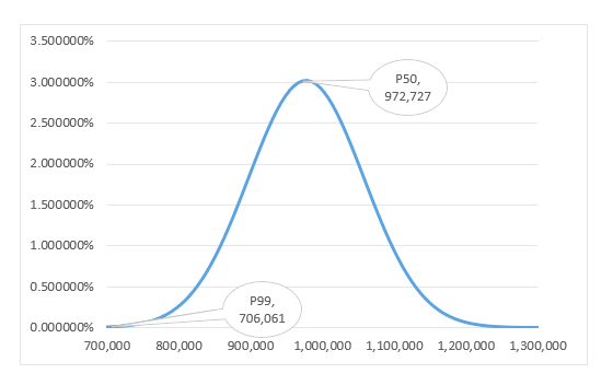
A couple times people have asked me to make a graph of the probability distribution. I struggled with this and in the attached file you can see how I made the graph below. You need the standard deviation and the P50 or average. Later in this page I describe how to compute the standard deviation using the mean squared error and assuming that different sources of variability are completely uncorrelated. Given the mean and standard deviation, you can first compute a minimum and maximum with the NORMINV function and a very small and a very large probability. Then you can make a range of values between the minimum and maximum. Once you have the values, make and x-y graph using the values as the x-scale and use the NORMDIST function as the y-scale. When you use the NORMDIST function, make sure the values add to 1.0. You may have to normalise the values through dividing by the sum. You can change the distribution and get a new graph and add P90 and a lot more stuff.
.
.
.
Review of Actual Studies
Before discussing some of the mechanics of computing P90, P95, P75 etc. for solar I review a few actual studies so you can see what kind of variation to expect between the lowest case (the P99 or P90 case) and the base case. I think it is good to compute the percent difference between the cases. In the first table that my friend Mijalo gave me from the internet, I show a table of variation in solar irradiation. The variation in solar irradiation is not the same as the variation in power production because it does not include variation from modelling uncertainty. The combined uncertainty is presumably the standard deviation divided by the mean. Note that the P90 one year in the Direct Normal Table is 88% and the 25 year variation is 90.86% (1850/2036).

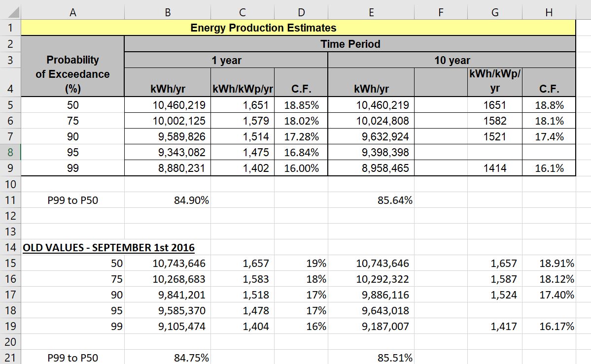
In the case below, the P99 to the P50 is 84% which is similar to the first table. If there were no fixed costs, you could use the formula % change = (DSCR-1)/DSCR. This can be converted to the required DSCR: % change * DSCR = (DSCR-1); % change * DSCR – DSCR = 1; % change * (DSCR – 1) = 1; (DSCR -1)= 1/ % change; and finally, DSCR = 1/%change – 1; or DSCR = 1/% change – %change/%change; or DSCR = (1-% change)/%change. So if you plug in 84%, you get DSCR = 1/.84% = 1.19.
The next extract is from a poorly structured model where the P90 title is wrong. But you can compare the P95 to the P50 case which is only 87%. This suggests a small DSCR is acceptable. Note the very high capacity factor in this case.
The next excerpt illustrates the change in production over a long period from degradation. In this case the 1-year p99 case is 88% of the P50 case.

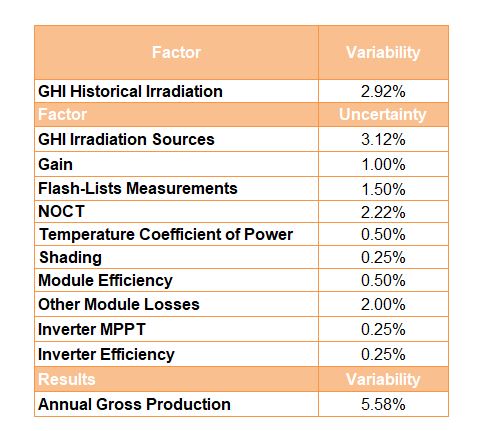
This table illustrates alternative sources of uncertainty. With the total uncertainty, you can compute the P90 can other cases. The sum of the uncertainty should be compute with the MSE as described below.
First Step: Computing Uncertainty from Historic Variation in Irradiation Data and Using NORMINV Function
In this section I have tried to take the mystery out of computing P90, P75 etc. The resource analysis section address issues with fundamental calculations of solar yield, performance ratios and temperature coefficients. To compute uncertainty and P values from historic data, you should first compute the average and standard deviation in annual energy. Then, you can use the NORMSINV function to compute the implied energy production that is given by different probability estimates.
The file that you can download below demonstrates how you can compute P90, P99, P75 etc. for weather uncertainty. Data is taken from the EU website (that is better than the Canadian and US sites). A link to the EU website that allows you to download historic solar energy data over long periods is below. A file that illustrates the calculation of standard deviation for weather variation and P values is available for download by clicking on the button below the link.
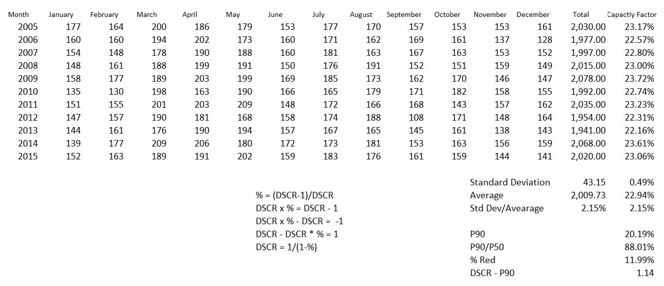
The screenshot below demonstrates how to compute standard deviation and P levels from data in the EU website. This page is part of the file available for downloading below. By downloading data for different years (from the monthly option), you can compute the standard deviation of solar energy and capacity factor. The P90 is computed with a value of 10% and the standard deviation and the mean. The percent reduction from the mean (P50) and P90 is 11.99%. This would justify a DSCR of 1.14.
The video below explains how to go to the EU website and convert data to excel so you can do analysis similar to the stuff in the above screenshot.
.
respect to historic weather data (e.g. cloud variation from year to year) is pretty easy. But that is not the only uncertainty. Computing the variation to to modelling errors and estimation of uncertainty in the potential modelling error and in the performance ratio is more difficult. On this page I explain some of the statistical ideas in computing uncertainty. Putting the uncertainty estimates together can be done by understanding the mean square error concept.
I have separated the analysis of solar resource into computing capacity factor or solar yield and the evaluating uncertainty around the base solar resource estimate. In analysing solar uncertainty, computation of P90, P95, P75 etc. is explained for solar power. Hopefully, I explain the solar resource uncertainty analysis and computation of P90, P99, P75 etc. without unnecessary complex statistical or technical terms. There are a lot of solar pages related to the files and the methods described below.
- The featured solar model page that is linked to this sentence includes completed finance models.
- There is also a file that allows you to automatically download panel prices and the price of silicon used in manufacturing the panels which is linked to this sentence.
- There is a webpage that works through resource issues including the performance ratio and how to find the best data on solar energy that hits a panel.
- There is a webpage that describes computation of the P50 versus P90, P99 etc. with some examples.
- There is a webpage that describes the arcane tax equity aspects of financing tax equity in the U.S.
- There is a page that works through how to consolidate multiple roof-top installations into a aggregate file.
Review of Actual Studies
Before discussing some of the mechanics of computing P90, P95, P75 etc. for solar I review a few actual studies so you can see what kind of variation to expect between the lowest case (the P99 or P90 case) and the base case. I think it is good to compute the percent difference between the cases. In the first table that my friend Mijalo gave me from the internet, I show a table of variation in solar irradiation. The variation in solar irradiation is not the same as the variation in power production because it does not include variation from modelling uncertainty. The combined uncertainty is presumably the standard deviation divided by the mean. Note that the P90 one year in the Direct Normal Table is 88% and the 25 year variation is 90.86% (1850/2036).
In the case below, the P99 to the P50 is 84% which is similar to the first table. If there were no fixed costs, you could use the formula % change = (DSCR-1)/DSCR. This can be converted to the required DSCR: % change * DSCR = (DSCR-1); % change * DSCR – DSCR = 1; % change * (DSCR – 1) = 1; (DSCR -1)= 1/ % change; and finally, DSCR = 1/%change – 1; or DSCR = 1/% change – %change/%change; or DSCR = (1-% change)/%change. So if you plug in 84%, you get DSCR = 1/.84% = 1.19.
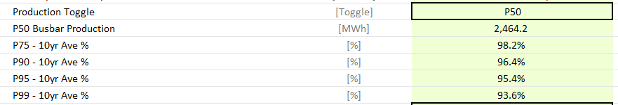
The next extract is from a poorly structured model where the P90 title is wrong. But you can compare the P95 to the P50 case which is only 87%. This suggests a small DSCR is acceptable. Note the very high capacity factor in this case.
The next excerpt illustrates the change in production over a long period from degradation. In this case the 1-year p99 case is 88% of the P50 case.
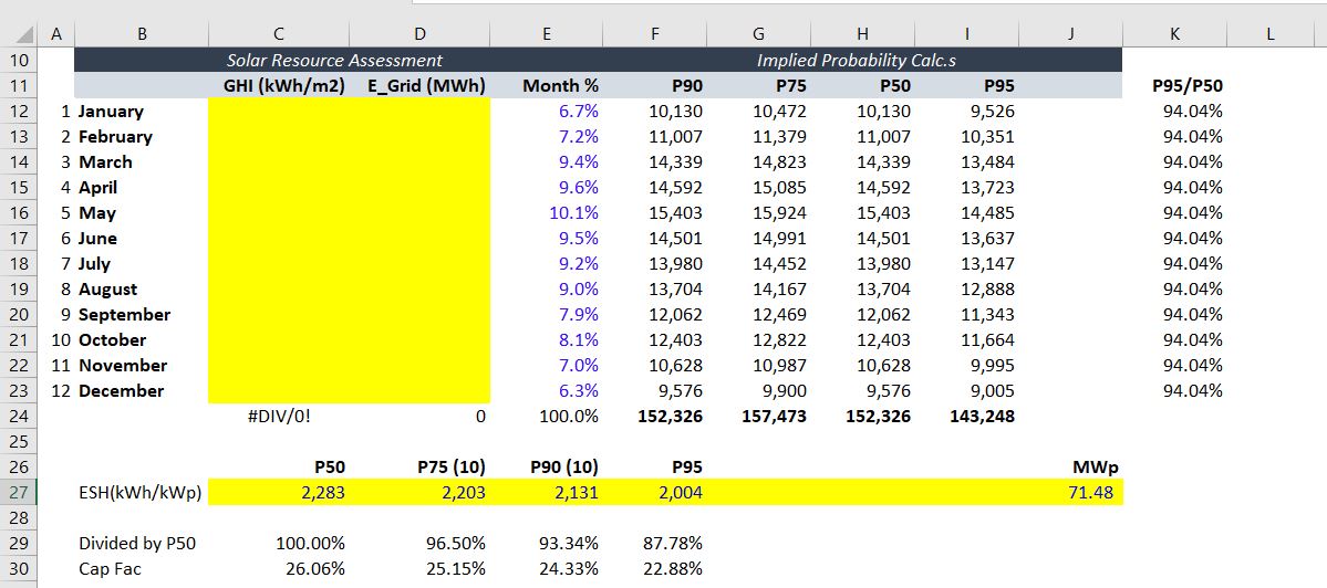
This table illustrates alternative sources of uncertainty. With the total uncertainty, you can compute the P90 can other cases. The sum of the uncertainty should be compute with the MSE as described below.
First Step: Computing Uncertainty from Historic Variation in Irradiation Data and Using NORMINV Function
In this section I have tried to take the mystery out of computing P90, P75 etc. The resource analysis section address issues with fundamental calculations of solar yield, performance ratios and temperature coefficients. To compute uncertainty and P values from historic data, you should first compute the average and standard deviation in annual energy. Then, you can use the NORMSINV function to compute the implied energy production that is given by different probability estimates.
The file that you can download below demonstrates how you can compute P90, P99, P75 etc. for weather uncertainty. Data is taken from the EU website (that is better than the Canadian and US sites). A link to the EU website that allows you to download historic solar energy data over long periods is below. A file that illustrates the calculation of standard deviation for weather variation and P values is available for download by clicking on the button below the link.
http://re.jrc.ec.europa.eu/pvg_tools/en/tools.html
The screenshot below demonstrates how to compute standard deviation and P levels from data in the EU website. This page is part of the file available for downloading below. By downloading data for different years (from the monthly option), you can compute the standard deviation of solar energy and capacity factor. The P90 is computed with a value of 10% and the standard deviation and the mean. The percent reduction from the mean (P50) and P90 is 11.99%. This would justify a DSCR of 1.14.
The video below explains how to go to the EU website and convert data to excel so you can do analysis similar to the stuff in the above screenshot.
[wonderplugin_video iframe=”https://www.youtube.com/watch?v=mIS5hkXx5I0″ videowidth=600 videoheight=400 keepaspectratio=1 videocss=”position:relative;display:block;background-color:#000;overflow:hidden;max-width:100%;margin:0 auto;” playbutton=”http://edbodmer.com/wp-content/plugins/wonderplugin-video-embed/engine/playvideo-64-64-0.png”]
Second Step: Adding Uncertainty in Performance Ratio and Modelling Uncertainty
Uncertainty from modelling errors — maybe the solar estimation is biased; maybe the panels will not produce the correct output; maybe the PVSYST model has something wrong etc. are very different from uncertainty due to weather estimation. Weather estimation is mean reverting. This means when you have an error because of something like a long rainy season in one year, that the next year will probably move back to the average.
Putting the Uncertainties Together — You Cannot Add Uncertainty; Use Mean Squared Error Instead
You should be able to (1) find a base yield from looking at the websites; (2) review long-term hourly solar data and compute the P90 and P99 that arises from variation in solar irradiation from year to year (due to clouds and dust); (3) add uncertainty related to the performance ratio and use the mean squared error to develop final P90, P99 etc.; and, (4) examine historic data for actual projects and understand the difference between actual observed variation and variation that is possible before the project begins. A separate spreadsheet is provided if you want to evaluate your skills.
In the spreadsheet that you can download below, I prove that when you square the standard deviation (to get the variance) and then add up the variance and take the square root of the sum of variances that this does measure the standard deviation of the combined factors. This works when the combination of factors is independent of each other. Let’s put the stuff together separately:
- Compute the standard deviation of the variation in production from each of the factors. For example, assume the standard deviation of the gross production before accounting for the performance ratio is 1,000. Assume that this has a standard deviation of 2.5%. Assume that the performance ratio is 80% and it has a standard deviation of 5%. The standard deviation of the gross production is 25 and the standard deviation of the performance ratio is 200 x 5% or 10.
MSE Simulation.xlsm
[wonderplugin_video iframe=”https://www.youtube.com/watch?v=m7RzDbHkM-k” videowidth=600 videoheight=400 keepaspectratio=1 videocss=”position:relative;display:block;background-color:#000;overflow:hidden;max-width:100%;margin:0 auto;” playbutton=”http://edbodmer.com/wp-content/plugins/wonderplugin-video-embed/engine/playvideo-64-64-0.png”]
Uncertainty Analysis from Variation in Actual Projects
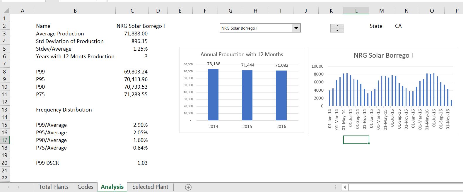
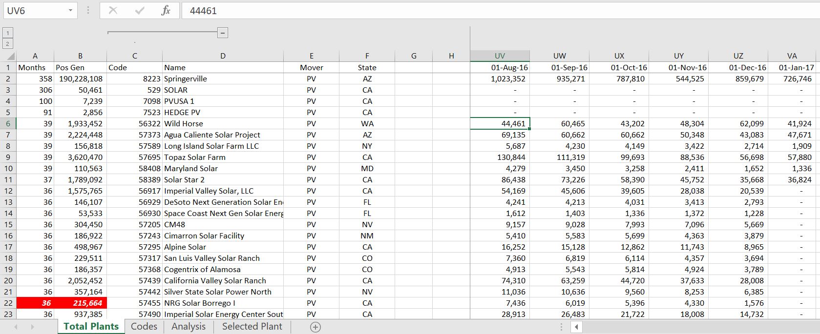
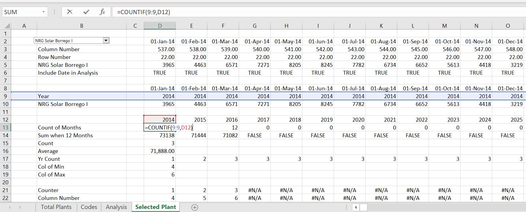
I have created a database that contains actual historic production data on operating solar projects. In the U.S. the EIA collects data on every power plant production by month (some plants do not seem to report as well as others). I have used the month by month data and converted the data to annual uncertainty in order to evaluate the actual year to year uncertainty. There are some natural problems with this analysis. First, the configuration of the project may change. Second, there are not a lot of projects with long-term data. I am in the process of adding capacity to the database so that you can evaluate the capacity as well as the production data. I have put a similar file in the wind analysis section and the hydro analysis section. The hydro section has much more data.
Subsequent lesson sets involve creating an analysing financial models. One deals with making a single project and another on making a portfolio of projects in a rooftop analysis.
Generation Database – Solar.xlsm
P99 etc Analysis.xlsx
Combined Analysis.xlsx
US Hourly Time Series Comparison.xlsm
Files with Historic Data to Compute Standard Deviation of Irradiation
I have also shown some data on historic solar data that is a good place to start. This was provided by NREL but they decided to stop providing the data.
Chicago.xlsm
Alaska.xlsm
Seattle.xlsm
Solar Resource Template.xlsm
Las Vegas.xlsm
Sources for Hourly Files with Details:


.
Second Step: Adding Uncertainty in Performance Ratio and Modelling Uncertainty
Uncertainty from modelling errors — maybe the solar estimation is biased; maybe the panels will not produce the correct output; maybe the PVSYST model has something wrong etc. are very different from uncertainty due to weather estimation. Weather estimation is mean reverting. This means when you have an error because of something like a long rainy season in one year, that the next year will probably move back to the average.
Putting the Uncertainties Together — You Cannot Add Uncertainty; Use Mean Squared Error Instead
You should be able to (1) find a base yield from looking at the websites; (2) review long-term hourly solar data and compute the P90 and P99 that arises from variation in solar irradiation from year to year (due to clouds and dust); (3) add uncertainty related to the performance ratio and use the mean squared error to develop final P90, P99 etc.; and, (4) examine historic data for actual projects and understand the difference between actual observed variation and variation that is possible before the project begins. A separate spreadsheet is provided if you want to evaluate your skills.
In the spreadsheet that you can download below, I prove that when you square the standard deviation (to get the variance) and then add up the variance and take the square root of the sum of variances that this does measure the standard deviation of the combined factors. This works when the combination of factors is independent of each other. Let’s put the stuff together separately:
- Compute the standard deviation of the variation in production from each of the factors. For example, assume the standard deviation of the gross production before accounting for the performance ratio is 1,000. Assume that this has a standard deviation of 2.5%. Assume that the performance ratio is 80% and it has a standard deviation of 5%. The standard deviation of the gross production is 25 and the standard deviation of the performance ratio is 200 x 5% or 10.
MSE Simulation.xlsm
[wonderplugin_video iframe=”https://www.youtube.com/watch?v=m7RzDbHkM-k” videowidth=600 videoheight=400 keepaspectratio=1 videocss=”position:relative;display:block;background-color:#000;overflow:hidden;max-width:100%;margin:0 auto;” playbutton=”http://edbodmer.com/wp-content/plugins/wonderplugin-video-embed/engine/playvideo-64-64-0.png”]
Uncertainty Analysis from Variation in Actual Projects
I have created a database that contains actual historic production data on operating solar projects. In the U.S. the EIA collects data on every power plant production by month (some plants do not seem to report as well as others). I have used the month by month data and converted the data to annual uncertainty in order to evaluate the actual year to year uncertainty. There are some natural problems with this analysis. First, the configuration of the project may change. Second, there are not a lot of projects with long-term data. I am in the process of adding capacity to the database so that you can evaluate the capacity as well as the production data. I have put a similar file in the wind analysis section and the hydro analysis section. The hydro section has much more data.
Subsequent lesson sets involve creating an analysing financial models. One deals with making a single project and another on making a portfolio of projects in a rooftop analysis.
Generation Database – Solar.xlsm
P99 etc Analysis.xlsx
Combined Analysis.xlsx
US Hourly Time Series Comparison.xlsm
Files with Historic Data to Compute Standard Deviation of Irradiation
I have also shown some data on historic solar data that is a good place to start. This was provided by NREL but they decided to stop providing the data.
Chicago.xlsm
Alaska.xlsm
Seattle.xlsm
Solar Resource Template.xlsm
Las Vegas.xlsm
Sources for Hourly Files with Details:
[wonderplugin_video iframe=”https://www.youtube.com/watch?v=mIS5hkXx5I0″ videowidth=600 videoheight=400 keepaspectratio=1 videocss=”position:relative;display:block;background-color:#000;overflow:hidden;max-width:100%;margin:0 auto;” playbutton=”http://edbodmer.com/wp-content/plugins/wonderplugin-video-embed/engine/playvideo-64-64-0.png”]