On this page I demonstrate how to use a load duration curve in computing the long-run marginal cost of electricity. The load duration curve can be used together with screening analysis to find the optimal capacity of different kinds of electricity plants. With the optimized run time, the long-run marginal cost can be evaluated.
The graph below demonstrates the general objective of the load duration and screening analysis. The graph inserts different types of capacity underneath the sorted load curve. The amount of capacity in different tranches depends on cost minimization when determining the capacity factors. The set-up of this graph is included in the spreadsheet for download below. The power point presentation that is available for download below the spreadsheet is the set of slides that describes all sorts of electricity economic issues including the development of long-run marginal cost from a load duration analysis.
Spreadsheet File with Load Duration Curve Exercise Using Entire Load Curve with 8760 Hours
Power Point Slides Used for Economic Analysis of Electricity Prices and Marginal Cost Analysis

The graph can also be used to evaluate the short-run and long-run marginal cost. The short term marginal cost is the running cost of each of the plant types for the different loads. The long-run marginal cost is the weighted average cost of the different types of units where the capacity cost is weighted by the amount of capacity and the energy cost is weighted average cost of running capacity for the amount of time it is running. Note that this is a somewhat simplistic analysis because reserve margins and cost of outages should be included in the analysis.
Step by Step Summary to Combine Screening Analysis and Load Duration Curves in Computing Long-Run Marginal Cost
To illustrate how to compute long-run marginal costs and estimated costs of energy in long-run equilibrium, you can follow the steps below:
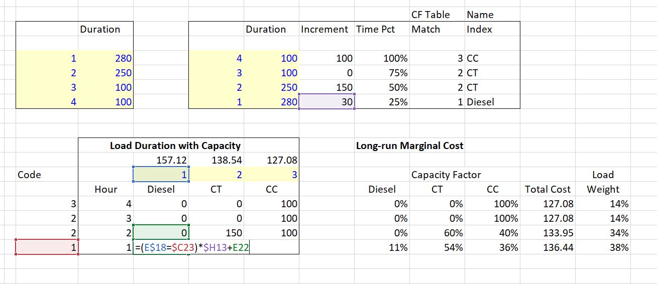
- Step 1: Create a load duration curve where you sort from the lowest value to the highest value (note that this is the opposite of a typical load duration curve).
- Step 2: Compute the overall capacity factor as the percent of time for each hour. This is a simple calculation where you count the hours and divide by 8760. For example, the second hour when you sort from low to high is 8759/8760 or more than 99%. A plant operating in this increment of load would have a capacity factor of more than 99%.
- Step 3: Once you have the capacity factor for each increment, use the lookup function to find the plant number that matches the capacity factor from the screening analysis. The screening analysis is discussed below and produces a list of plants that are optimal to run for different capacity factors.
- Step 4: Transpose the plants from the screening analysis to the load duration curve and put the code number for each plant at the top. Then make a switch for whether the plant is the incremental plant running. This switch is used by comparing the code number from step 3 above to the code number at the top of the page.
- Step 5: For each load value (e.g. 8760), compute the increment of the load and the accumulated percent of time at the particular load. For the minimum load or the first load value, the increment is the load itself. For subsequent higher loads, the incremental load is the load of the row you are on minus the previous load.
- Step 6: Compute the accumulated generation for each plant type. When the switch is true the generation is accumulated. When the switch is not true the accumulation stops.
- Step 7: Compute the marginal cost per hour. To do this you can use the lookup function again, but this time lookup against the variable cost from the screening analysis.
The first step is evaluating the fixed and variable costs of different types of options. You can refer to other parts of the energy analysis to evaluate important issues associated with carrying charge analysis. The screenshot below demonstrates various different possible addition options with different fixed and variable costs.
Once you have defined fixed and variable costs, you can compute the total cost per MWH at different capacity factors. The computation of different costs for different capacity factors is demonstrated in the screenshots below. The first screen shot illustrates that case of three plants with different fixed and variable costs. The IND/MTH in the bottom part of the screen shot stands for INDEX/MATCH and it shows the break-even capacity before which different plants are economic.
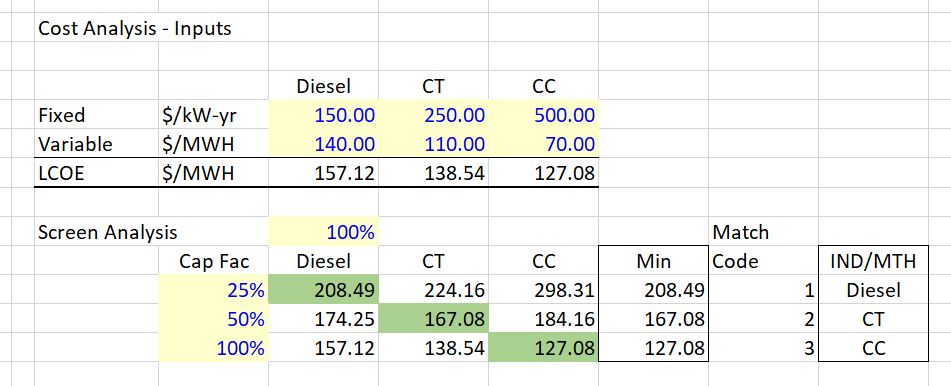
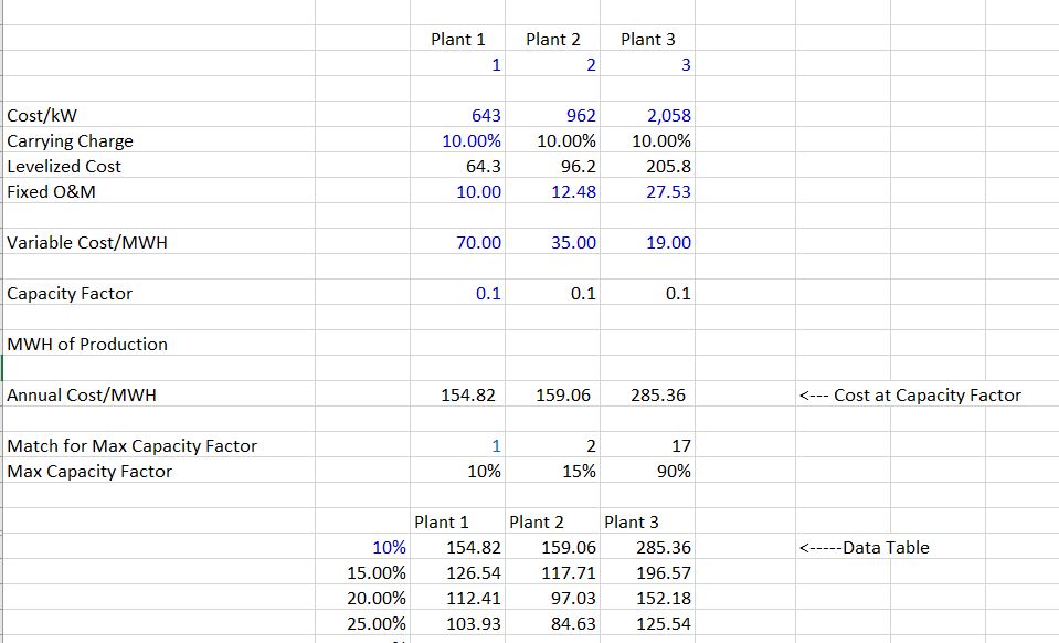
The graph below demonstrates how to compute screening analysis for the dispatchable capacity. The capacity factor is on the x-axis and the total cost including both fixed and variable cost is shown on the vertical axis. In the case below, the red line for Plant 2 is almost always optimal.
Computation of Optimal Capacity After Screening Analysis
Once you have computed the screening analysis, you can use the break-even capacity factors to fit the different types of capacity underneath a load duration curve. The first step is computing the time underneath the load duration curve beginning with the low part of the curve. Then you can match the break-even points with the various time factors.
Video on Load Duration Curve and Long-Run Marginal Cost
I am afraid the video below really sucks. But I have not bothered to make a new one and please do not make me feel bad by saying something OMG this makes no sense.
[wonderplugin_video iframe=”https://www.youtube.com/watch?v=hJ21Ie2NjIY” videowidth=600 videoheight=400 keepaspectratio=1 videocss=”position:relative;display:block;background-color:#000;overflow:hidden;max-width:100%;margin:0 auto;” playbutton=”http://edbodmer.com/wp-content/plugins/wonderplugin-video-embed/engine/playvideo-64-64-0.png”]
.
[wonderplugin_video iframe=”https://www.youtube.com/watch?v=8YP6FifxcVM” videowidth=600 videoheight=400 keepaspectratio=1 videocss=”position:relative;display:block;background-color:#000;overflow:hidden;max-width:100%;margin:0 auto;” playbutton=”http://edbodmer.com/wp-content/plugins/wonderplugin-video-embed/engine/playvideo-64-64-0.png”]
Long-term Equilibrium Analysis
The file you can download below demonstrates how to compute long-term supportable prices in a merchant market that will allow construction of new capacity. It is method that uses a peaker method to measure capacity and optimises costs from measuring the profit against merchant prices.
Spreadsheet File that Demonstrates how to Compute Long-term Equilibrium Prices with Peaker Method