This page discusses modelling techniques of computing sculpted debt repayments in the situation with an amount of debt given by the debt to capital ratio and a minimum DSCR. If three parameters are fixed: (1) the size of the debt; (2) the minimum DSCR; and, (3) the average debt life, then the optimal DSCR may not be constant over the tenure of the debt. This modelling problem of sculpting debt repayments to achieve an non-constant DSCR that is described on this page is one of the most difficult problems in project finance. The problem illustrates the use of formulas in modelling, using an interpolate function and carefully designing the structure.
When the average debt life, the minimum DSCR and the amount of debt are fixed, the period by period repayment cannot be easily calculated (as contrasted for example, in a sculpting case where the constant DSCR drives the debt level and a formula can be used for computing repayment). Specifically, if the DSCR changes over the tenure of the debt, the repayment pattern of the debt cannot be defined by a simple formula such as CFADS/DSCR. The only definite in the case with the size of debt given and a debt life constraint is that at some point over the debt tenure, the DSCR cannot fall below the minimum DSCR.
Three spreadsheets are used to explain the process of sculpting with fixed debt, a minimum DSCR and an average debt life constraint. The first spreadsheet assumes DSCR’s are given and the amount of debt is derived from the cash flow and the debt terms. In cases such as this, the aggregate DSCR and the total cash flow drives the analysis. In the second example, the debt size is given and the aggregate DSCR is derived from PV of the Aggregate Debt Service at the weighted average interest rate. The third spreadsheet includes sculpted debt repayment in the case where the DSCR gradually reaches the minimum debt DSCR and there are taxes that create a circular reference.
The big trick in solving these problems is an allocation issue. After aggregate total debt service is computed, the aggregate debt service is allocated to the non-flexible (other) debt issues using a formula where a sculpting ratio is computed from the amount of debt and the PV of Aggregate Debt service as shown below.
- PV of Debt Service from Aggregate
- Target Debt from Input
- Sculpting Ratio -> Debt/PV of Aggregate Debt Service
- Debt Service Allocated to Debt Issue – Aggregate DS x Ratio
.
The button below is the file that is assocated with the webinar and the video for the comprehensive example with different operating assumptions, and different debt sizing and then allocating debt service to different issues. I have included the button here so it may be easier to find.
.
.

.
Case 1: Given DSCR, Interest Rates and Tenures But Not the Aggregate Debt Amount
The first example attached to the button below demonstrates a case where a varying DSCR is given but the level of the aggregate debt is not given. Please note and think about this case — you cannot define the aggregate DSCR with drives the debt and the amount of debt at the same time. This is like the setting the debt size with a debt to capital ratio or a fixed amount of debt.
To complete this case, the following steps and concepts are used:
- From the input of the DSCR and the input of CFADS, compute the target Aggregate Debt Service.
- From the given debt amounts for the non-flexible issue, compute the PV of the Aggregate Debt service over the debt tenure and use this PV of debt service at the particuar rate to compute the allocation ratio defined above — PV of Debt Aggregate Debt Service/Given Debt.
- Use the aggreate debt service multiplied by the aggregate debt service to compute the debt service for the issue
- Do the same calcluations for other debt issues
- For the flexible debt issue with the longest tenure, compute the debt service as the Aggregate debt service less the debt issue from the flexible issues and compute the PV of the debt service.
- Put the debt service less the interest into separate debt issues and verify that the balance on each issue falls to zero.
Inputs to the model
Inputs to the model are shown in the two screenshots below. Note that the non-capture debt issue is derived and not input in this case and the DSCRs are input.
.

.

.
Debt Service on Non-Flexible, Non-Capture Debt Issues
The next step is computing the debt service for the non-capture debt issues using the allocation factor discussed above. This computation from the aggregate debt service is shown in the next screenshots. Note that the flag is necessary for computing the PV of the aggregate debt service at the tenure.
.

.
Debt Service on Flexible, Capturing Issue (After other Issues)
After the other debt issues, the flexible debt issue is calculated using the standard formula where Aggregate CFADS/Target DSCR = Aggregate Debt Service and Aggregate Debt Service less other Debt Service = Flexible Debt Service.
.

.
Debt Balances with Proof that the Method of Allocation Works
The debt balances for all of the issues are shown in the screenshot below. Note that for all of the debt issues, the debt balance goes to zero in the correct period.
.

.
Case 2: Debt is Given with Interest Rates and Tenures But Not the DSCR, which is Derived from Some Kind of Shaping Function
.
This case begins with given debt and derives the DSCR. It is important that you do not get into some kind of trap where you believe that you can be given the DSCR and the debt size and then allocate debt to multiple debt issues. In this case, the interpolate function is used to derive the shape of the DSCR. Other manual methods or shaping algorithms could be used.
In this case the inputs include the given amount of debt and the general shaping parameters of the DSCR sculpting function.
Inputs to the model
.

.
Compute the Non-Flexible, Non-Capture Debt Issues with Allocation Factor — Debt/PV of Aggregate DS
The next screenshot demonstrates that for the other non-flexible debt issues, the allocation formula using the PV of the aggregate debt service divided by the fixed debt amount. It is just the same as the first example.
.

.
Debt Service on Non-Flexible, Non-Capture Debt Issues
The next screenshot shows the computation of debt service for the remaining flexible debt issue. Note that this is necessary even if all of the debt tenure’s are the same. The debt service for the flexible issue is computed as the total aggregate debt service less the debt service on the other issues. The net present value of the debt service at the particular interest rate is the amout of debt and should be the same as the input debt.
.

.
The next screenshot demonstrates that when you compute the balance of the debt, the debt balance goes to zero at the end of the tenure of the debt.
.

.
The debt service for the different issues can be illustrated with a waterfall chart which is a stacked area chart. Note that you do not explicitly put the CFADS in the chart, but the remaining dividends so the stacking works.
.

.
Spreadsheet with Simple Sculpting Analysis Including Taxes with Goal Seek and Solver Tools
.
.
The discussion below deals with financial modelling issues associated with sculpting in the case of fixed debt and average loan life constraints. Other pages address theoretical issues and more technical discussion of how to develop user defined functions.
.
Base Calculations with No Taxes Using Solver and Goal Seek
In computing the debt repayment that does not have a constant DSCR, the following calculations are necessary before an optimise function is used:
- The LLCR should be computed from the net present value of CFADS divided by the amount of debt outstanding.
- Some kind of interpolation function can be used to move from a high DSCR (that allows more dividends) down to the minimum DSCR.
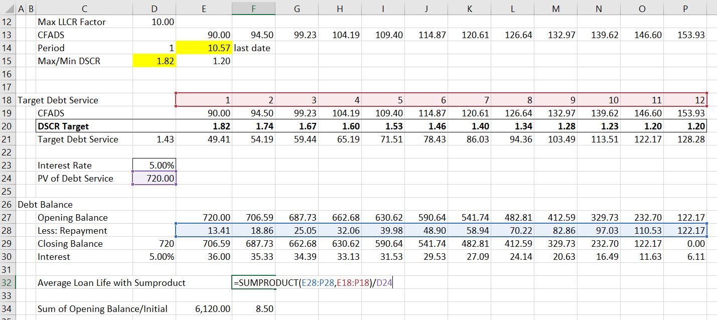
- The average loan life should be computed (using either the SUMPRODUCT function with repayments and debt period divided by the loan balance or the sum of the closing debt balance divided by the initial debt balance).
- The debt balance should be computed from the net present value of debt service.
- The initial DSCR can be computed from the LLCR computed in step 1 and a constant factor
- The interpolation between the intial DSCR and the minimum DSCR as well as the constant LLCR factor can be used to derive the DSCR interpolation.
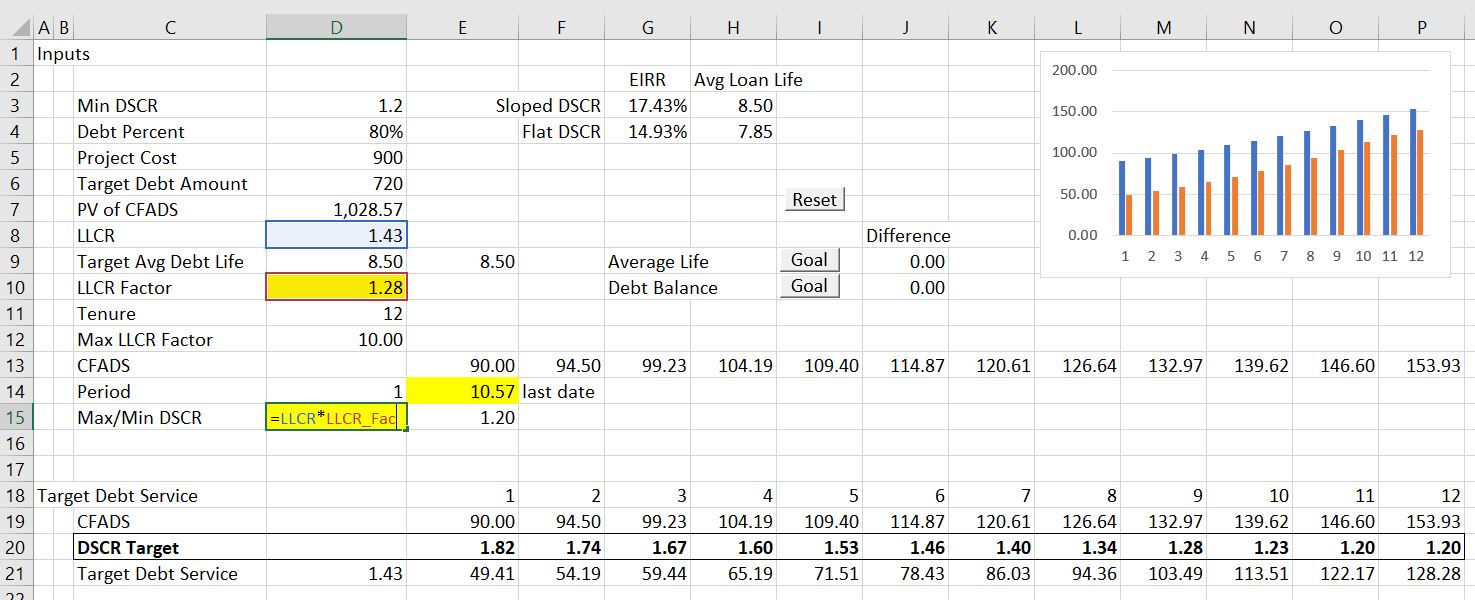
Some of the steps used to compute the interpolated DSCR are shown below. The first screen shot demonstrates how the LLCR can be used if the DSCR is constant. The LLCR is the PV of the CFADS of 1,028 divided by the constrained debt of 720. Since the LLCR is equal to the DSCR when the DSCR is constant throught the debt life, the LLCR can be used to produce a constant DSCR over the debt term with sculpting:
.
Case 1: Fixed Debt Size with Flat DSCR
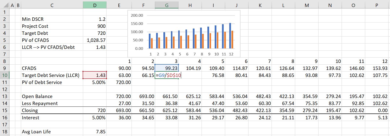
This basic case which is used in various other cases is founded on the idea that the PV of CFADS divided by the DSCR gives the value of the debt. This notion that PV(CFADS)/DSCR = Debt, can be reversed giving the formula:
LLCR = PV(CFADS)/Debt
As the DSCR is constant, DSCR = LLCR and the debt service can be given by the formula below:
DS = CFADS/LLCR
PV of DS = Debt
The formula below is illustrated in the excerpt from the spreadsheet below. The debt service in row 10 is computed as the CFADS divided by the computed LLCR. In this case, the minimum DSCR is not ever in place. Note that the minimum DSCR is 1.2 and, the LLCR of 1.43 is used as the basis for computing a debt service. This produces a DSCR that is constant throughout the tenure of the debt. The debt balance table demonstrates that the closing balance of the debt goes down to zero by the end of the debt life.
.
.
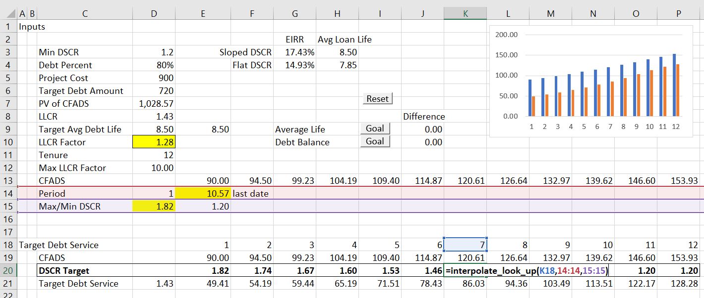
In the second screenshot, the interpolate function (UDF) is used to move the DSCR from a high level down to the minimum level. In this case, the DSCR begins at 1.82 and by year 11 it falls to the minimum level of 1.2. With these DSCR’s, the total debt is equal to the target debt of 700. The interpolate function is described in detail in the Excel Utilities section of the website. You can download the interpolate function file and copy the function to your project finance modelling file.
.
.
The third screen shot shows calculation of the average loan life. There are two methods to compute the average loan life. The first is using the SUMPRODUCT function and the second is using the sum of the closing balance divided the balance of the debt. The average debt life is necessary to compute because the average debt life is a constraint on the pattern of repayment.
.
.
The next screen shot demonstrates how the interpolation factors can be computed. The first factor is the final period before which the minimum DSCR is applied. The second factor is the LLCR as computed above multiplied by an LLCR factor. By changing both the final period and the LLCR factor, the progression of the DSCR over time can be changed. This change in the progression of the DSCR affects both the level of the debt and the average debt life.
.
.
While the solver tool can seem to be the ideal solution to the sculpting problem, there are a number of problems that include:
1. When alternative starting points are used, the solver does not work and a message that states a solution could not be found arises. For example if you enter the LLCR factor as 0.5, the solver fails to find a solution. A similar problem where the solver does not work occurs when the LLCR factor has a high value of something like 30.
2. If taxes are included in the analysis, there is an additional constraint driven by the circular reference from the interest deduction in computing taxable income. Specifically, the issue is related to computing the LLCR from PV of CFADS divided by target debt. To solve the problem, (1) the PV of CFADS can be fixed; (2) the fixed amount of PV is compared to the computed amount; and, (3) a solver equation can be added to set the difference to zero by changing the fixed amount. When the circular reference constraint is added to the end time and the LLCR factor constraint, the solver function is less stable as shown on the second screenshot below.
3. To address circular references in a comprehensive manner it may be clumsy to use the solver. For example, the tenure may change, DSRA income or DSRA L/C fees may have to be included and a host of other details can arise. Many of these factors related to the DSRA can cause circular reference problems and require changing the set-up of the solver. These issues may result in the solver failing. For this reason, I have created a user defined function that replicates in a crude manner what the solver does.
4. In attempting to find a pattern of DSCR ratios that produce the target average life and the correct debt balance, there are situations where a solution is not possible. One example is when the target debt life is impossible to obtain with the tenure, minimum DSCR and the interest rate. A second example is when the average debt life is less than the debt life that would be produced by a simple LLCR technique. In both or these situations the solver will continue iterating and will not work. The problem is that you may not necessarily know why.
The screenshot below illustrates a case where the solver is not working. In this example note the extreme initial DSCR which occurs after the solver has clunked along for a long time.
User-Defined Function to Optimise Debt Life and Debt Amount with Curved DSCR
Rather than use the solver or goal seeks, I have made a UDF to optimise the DSCR and debt repayment. In mimicking the solver, the iteration process is more tricky than creating a couple of dynamic goal seek functions. To think about how the UDF works, you could use the simple example and press goal seek, then manually adjust the LLCR factor in the correct direction. Then you could press the goal seek again and again adjust the LLCR factor. You could keep doing this until both the average debt life is equal to the target debt life and the debt balance equals the target debt balance driven by the debt to capital ratio.
If you are working on this sculpting problem, I recommend that you open the file and try to experiment with different parameters. I should not say this because I think it is absurd to compare financial modelling with art, but when messing around with different cash flow patterns, minimum DSCR’s, target loan lives, debt to capital ratios etc., you can immediately see the effects on the DSCR, the repayment structure and the equity IRR. I hope you try it even if you don’t understand all of the technical or even financial issues and understand what a financial model should really do.
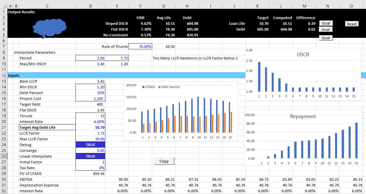
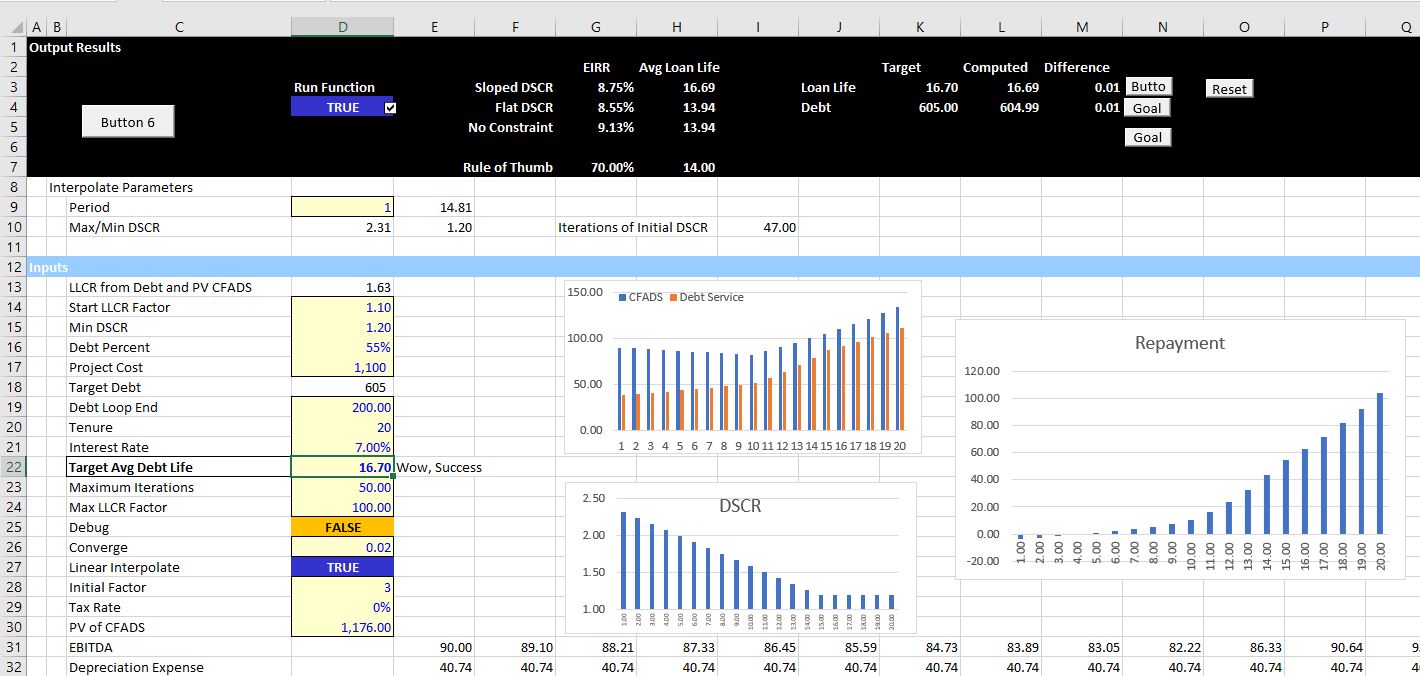
A few illustrations of how the UDF works are demonstrated in screenshots below. The first screenshot demonstrates the general output of the UDF in a scenario where there are no problems with the iteration process. In this case there is a little note stating that the process has worked. You can change various parameters including the average debt life, the minimum DSCR and the debt size and evaluate the change in repayment patterns.
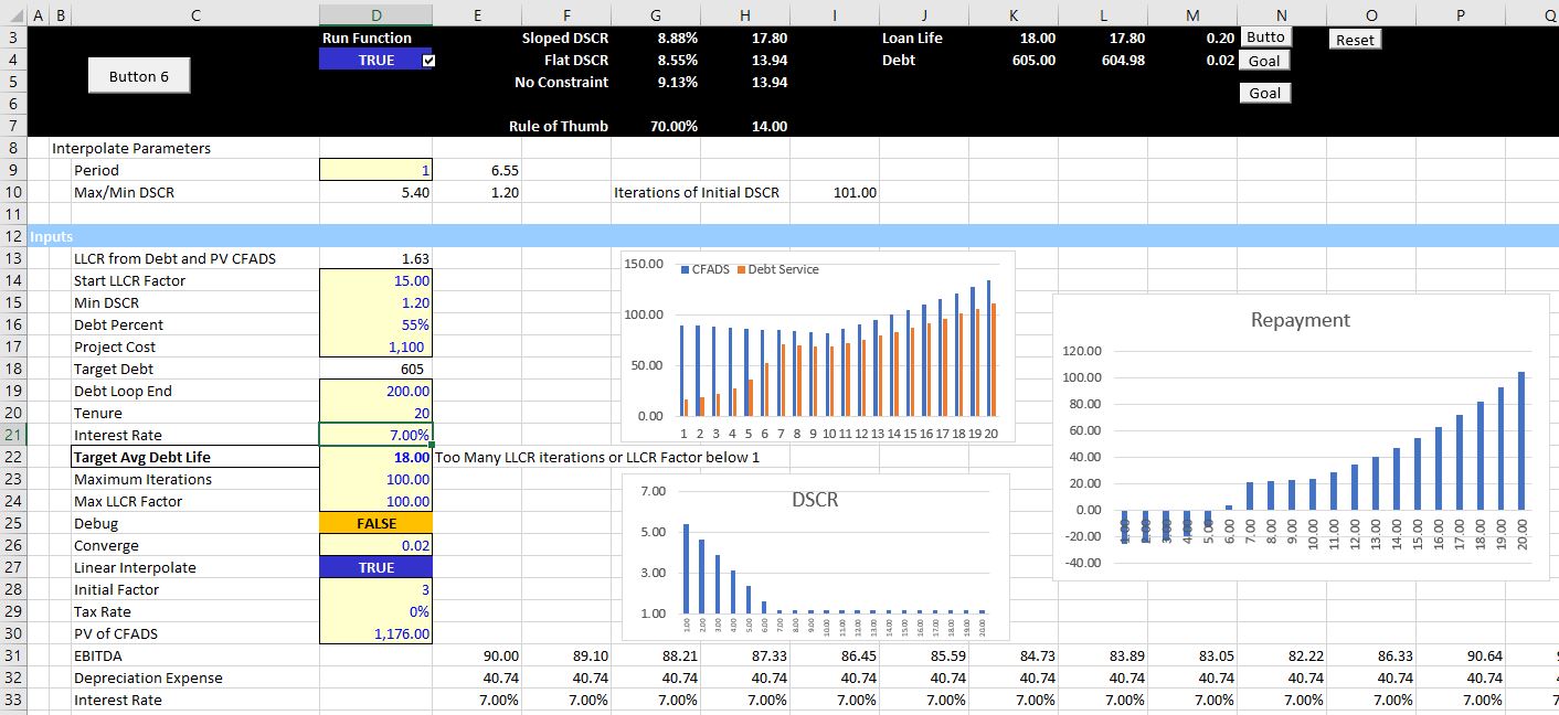
A second case is demonstrated in the screenshot below where success is not obtained. You can think about things that will make the process not work. One example is where the LLCR and the Minimum DSCR are close to one another. In this case, trying to make the average debt life longer than the average life from flat case will not work. A second extreme example is when attempting to make the average debt life longer than is possible from the shape of the repayment curve. There is a limit on the debt life relative to the debt tenure — if all the repayment occurs at the last year, then the average life will be equal to the tenure. This situation where the tenure is equal to the average life of course is not possible because of the DSCR constraint, but the example does illustrate the constraint on too long a debt life. The screenshot below demonstrates that when you make the target debt life too long, the iterative process cannot find a solution. But unlike the solver process, the lack of solution is clearly presented and you can quickly adjust different parameters to find better inputs. The screenshot also shows that in extreme cases there is negative amortisation which will probably be unacceptable to the financial institution.
.
Changing the Function to a Macro to Verify the Iteration Routine
It has been painful to develop methods that will perform the iterations in an efficient manner and not result in a continual loop. You may want to inspect the iteration process yourself and see if you can find parameters to make the process more efficient. I hope this does not ever occur, but the function could result in an infinite loop. To allow you to inspect the iteration process, I have made the function so that you can convert it into a macro. When you convert the function to a macro, the various ways in which the goal seek loop for solving the debt balance and the LLCR factor iteration for solving the average life are documented. The documentation is printed on a separate spreadsheet page.
If you would like to run the macro you have to change a couple of items in the code. You should remove the single inverted comma (‘) next to the function name. You should also remove the single inverted comma from the Sub name. Finally you should change the function name variable from true to false in the code. The code below illustrates how the items that you should change. The first excerpt shows the code in the function mode. The second excerpt shows the code in the macro mode.
To run the macro you can press the little cloud symbol at the top left of the spreadsheet as illustrated in screenshot below. If the inputs for debt life, minimum DSCR, debt tenor, debt size and EBITDA are the same (and the tax rate is zero), then the function and the macro should produce the same results. But if you run the macro, you can see details of how the process is converging and whether there are too many iterations or the process is bouncing back between variables.