This webpage explains how to model the amount of energy produced by a hydro plant when the plant can store water in a reservoir. The hydro plant has constraints on the amount of energy and the amount of capacity. Determining the amount of energy to release depends on value of energy at different time periods. Assuming that the value of energy is directly related to the size of the load, an optimisation process is easy to accomplish using the goal seek tool. To compute peak shaving you can start with the basic load. Then you put in an arbitrary set point which is the amount of load that is present before which the water is released. If load is above the set point, energy is produced by the hydro plant. You can sum the amount of energy using the set point. Then you can make sure that the sum of the energy produced by the hydro plant is equal to the energy available. You should also make sure that the capacity of the generator is not exceeded in any hour. My good friend Tom Vesalka has taught me this.
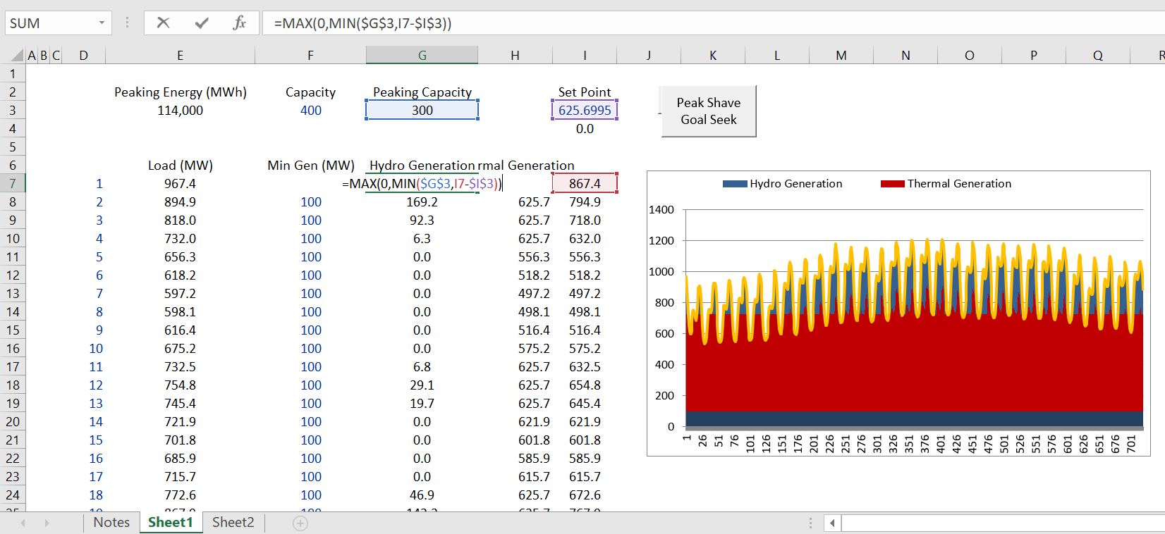
The peak shaving algorithm is demonstrated in the file that you can download by pressing the button below. There are just a couple of equations and a goal seek function. You need a maximum function with the load relative to the hydro generation and to make sure the hydro generation is not negative. For this you can use a MIN and MAX together as shown on the screenshot below.
.
.
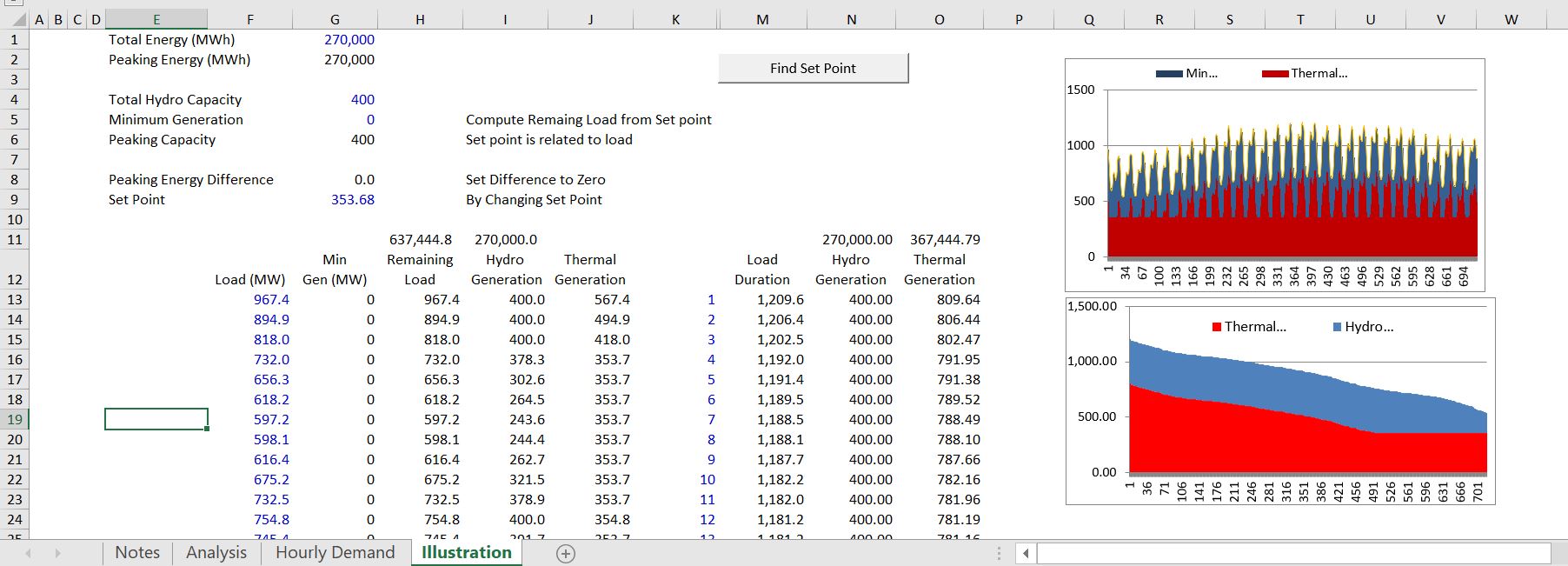
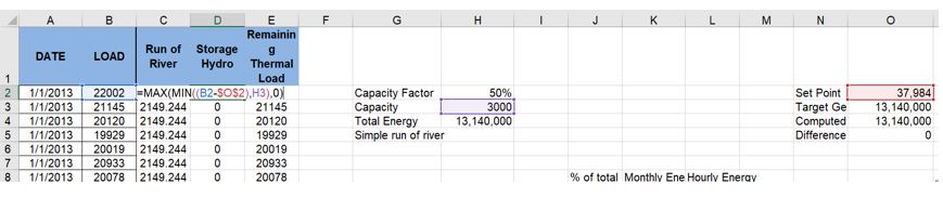
The process of using a goal seek function to find the set point is illustrated in the screenshot below. You can compute the difference between the computed generation from the hydro plant and the amount of energy available. This difference should be zero. To get the difference to zero you should also make an equation with the minimum function which assures that the generation cannot exceed the capacity of the generator. You need to first define the capacity factor and the capacity of the hydro project. The production in any hour cannot exceed the capacity and it should be limited by the set point. In the example below the set-point is in Cell I3. The capacity factor is defined by the amount of energy which is used in a goal seek. The goal seek process is illustrated in the second screenshot below.
The goal seek macro is simple as illustrated below. You should name ranges and record a macro.
.

Sub peak_shave()
'
' peak_shave Macro
'
Range("difference").GoalSeek Goal:=0, ChangingCell:=Range("set_point")
End Sub
The screenshot below illustrates how you can use the MIN and MAX and a set point to compute the total energy when you are peak shaving.
The computation of peak shaving is demonstrated in the file that you can download by pressing the button below.
Spreadsheet with Exercise on Hydro Peak Shaving with Constraints on Energy and Capacity
.
Peak Shaving and Solar Power
The method of peak shaving the portion of hydro that is flexible (assuming some is constrained by minimum levels) can work well with solar power and limit the use for batteries to resolve ancillary service issues. If you put solar power in the system it does not change the amount of power that can be generated does not change, but you can produce power in the evening rather than in the day time with the flexible hydro. To model this you can use the gross electricity load by hour (or a smaller increment) and then subtract the hour by hour solar. You can use PVGIS to compute the hour by hour solar. I label this as net load in the screenshots below. The file that includes the data on solar and hydro is included in the button below.
.
.
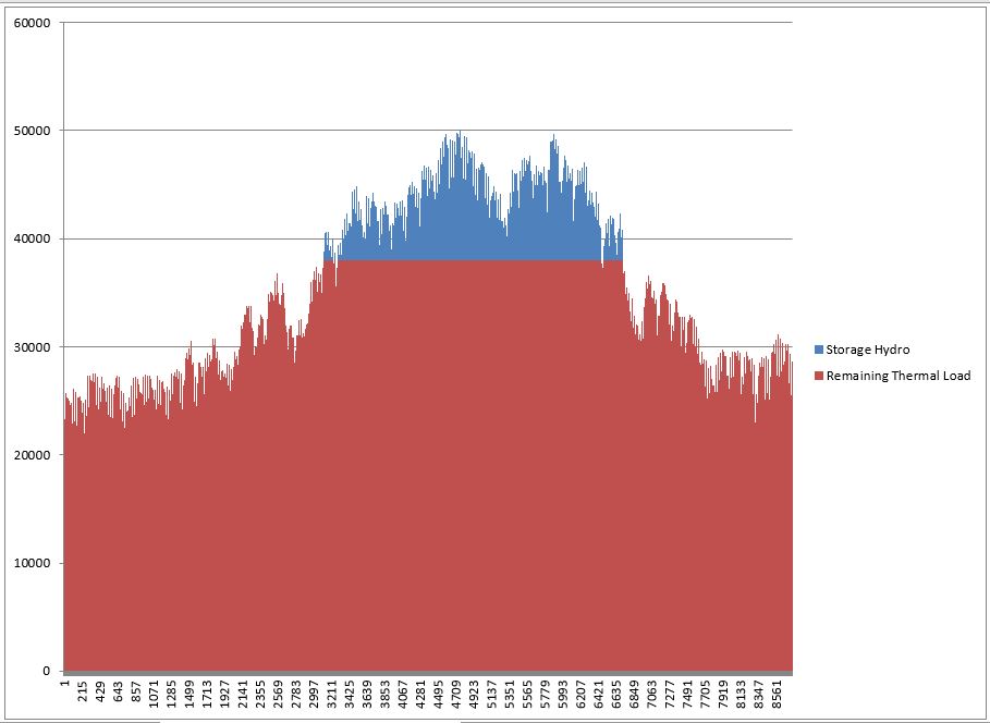
In the first screenshot we show a case without any solar and without peak shaving. To illustrate this I have made the total amount of energy to be constant as the minimum. There are two graphs on the picture. The left graph shows the load and the hydro for a week. The second screenshot shows the results for a single day. The graph aggregates the load and shows the load from thermal and the load from hydro. With the flat hydro the thermal power is not flat. When the thermal is not flat, the operators of the thermal complain.

.
If the minimum hydro is changed to zero allowing the hydro to fluctuate (the total generation is the same), then the thermal in the right-hand side graph is flat. This principle will be used in analyzing the solar production.
.

.
If solar is implemented as illustrated in the screenshot below (using PVGIS as explained in other pages), the solar is different for different months. The graph which is part of the file attached to the blue button above, allows you to evaluate the thermal production with different hydro production.

.
If this solar pattern is applied to hydro to compute a capacity factor (see the calculations in the solar section), then if the hydro is computed with the minimun non-flexible hydro, then the classic duck curve occurs and the hydro production is negative in sunlight hours (meaning if you have flat hydro production you cannot use all of the hydro and the solar). You could use a battery in this case.
.

.
When the hydro is flexible, the thremal load is flat. This is the big advantage of solar together with solar. Hopefully you can see the higher volatlity in net loads from solar with the very low levels of net load
.
